FLUENT - Supersonic Flow Over a Wedge- Step 6 *New

Step 6: Analyze Results

Plot Velocity Vectors

Let's plot the velocity vectors obtained from the FLUENT solution.

Display > Graphics and Animations or Results > Graphics and Animations

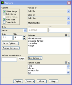
Select Vectors, click on the Set up  button. Under Color by, select Mach Number in place of Velocity Magnitude since the former is of greater interest in compressible flow. The colors of the velocity vectors will indicate the Mach number. Use the default settings by clicking Display.

This draws an arrow at the center of each cell. The direction of the arrow indicates the velocity direction and the magnitude is proportional to the velocity magnitude (not Mach number, despite the previous setting). The color indicates the corresponding Mach number value. The arrows show up a little more clearly if we reduce their lengths. Change Scale to 0.2. Click Display.

Zoom in a little using the middle mouse button to peer more closely at the velocity vectors.

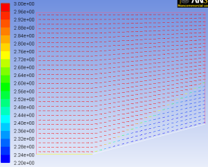
We can see the flow turning through an oblique shock wave as expected. Behind the shock, the flow is parallel to the wedge and the Mach number is 2.2. Save this figure to a file:

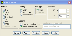
Main Menu > File > Hardcopy

Select JPEG and Color. Uncheck Landscape Orientation. Save the file as wedge_vv.jpg in your working directory. Check this iimage by opening this file in an image viewer.

Let's investigate how many mesh cells it takes for the flow to turn. To turn on the mesh do the following:

Display > Graphics and AnimationsorResults > Graphics and Animations

Select Vectors, click on the Set up button. Under options select the Display Mesh checkbox and a new window will pop up. Under Surfaces select default-interior,click Displayand close it.  

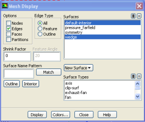
The mesh will substitute the arrows and to display both the mesh and the arrows go back to the Vector Set up window click Display again and now the mesh and arrows will appear on the same picture.

We see that it takes 2-3 mesh cells for the flow to turn. According to inviscid theory, the shock is a discontinuity and the flow should turn instantly. In the FLUENT results, the shock is "smeared" over 2-3 cells. In the discrete equations that FLUENT solves, there are terms that act like viscosity. This introduced viscosity contributes to the smearing. A more thorough explanation would have to go into the details of the numerical solution procedure.

Plot Mach Number Contours

Let's take a look at the Mach number variation in the flowfield.

Display > Graphics and Animations or Results > Graphics and Animations

Select Contours, click on the Set up  button. Under Contours of, choose Velocity.. and Mach Number. Select the Filled option. Increase the number of contour levels plotted: set Levelsto 100.

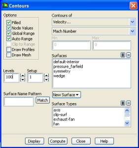
Click Display.

We see that the Mach number behind the shockwave is uniform and equal to 2.2. Compare this to the corresponding analytical result.

Plot Pressure Coefficient Contours

Pressure Coefficient is a dimensionless parameter defined by the equationwhere p is the static pressure,

P_ref is the reference pressure, and

q_ref is the reference dynamic pressure defined byThe reference pressure, density, and velocity are defined in the Reference Values panel in Step 5.
Let's set the reference values necessary to calculate the pressure coefficient.

Report > Reference Values

Select pressure-farfield under Compute From.

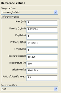
The above reference values of density, velocity and pressure will be used to calculate the pressure coefficient from the pressure.

Display > Graphics and AnimationsorResults > Graphics and Animations

Select Contours, click on the Set up  button. Select Pressure... and Static Pressure from underContours Of. Then select Pressure Coeffient.

The pressure coefficient after the shockwave is 0.293, very close to the theoretical value of 0.289. The pressure increases after the shockwave as we would expect.

Now we will plot the pressure coefficient along the wedge. Go to:

Results (left-hand side of the screen) > Plots

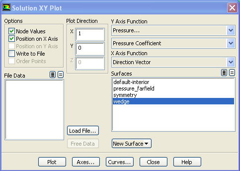
Select XY Plot and then click on the Set up button. In the pop-up window specify the Y Axis Function topressure and pressure coefficient. Select thewedge from the available surfaces and click Plot.Your specifications should look like the picture below.

The picture above, though descriptive might not give you the details you are looking for. You can save the data used in this plot to a file by checking the Write to File checkbox under  Options. Then click the Write... button, give the file a name and click Function.

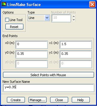
To measure the Shock Angle we can add a new line to the plot. Click on New Surface and select the Line/Rakeoption. Set the first point to (0,0.35) and the second one to (1.5,0.35) name the line y=0.35 and click on Create.

The new line will be added to the available surfaces. From these select Symmetry, Wedge and y=0.35. You will notice that there is no Plot button, this happened because the Write to file checkbox under options is still checked. Uncheck it and then click on Plot. You will now be able to see the lines on the plot.

Nest, we will plot the Total Pressure. To achieve this on the Solution XY Plot pop-up window select Total Pressure under Y Axis Function and click Plot.

Finally, we will find out what the drag coefficient for this scenario is. Close the pop-up window if it's still open and go to

Problem Setup > Reference Values

Make sure that the parameter for Area is 1.  Then go to

Results > Reports > Forces > Set up... > Print

The drag coefficient should be the value listed in the last column of the values in the output window.

Go to Step 7. Verification

See and rate the complete Learning Module

Go to all FLUENT Learning Modules