 Sign-up for free online course on ANSYS simulations!
Step 8: Postprocess the Results
Plot Deformed Shape
Main Menu > General Postproc > Plot Results > Deformed Shape
Select Def + undef edge and click OK.
This plots the deformed and undeformed shapes in the Graphics window. The maximum deformation DMX is 0.026148 inches as reported in the Graphics window. We should check that our results make sense. It appears that the boundary conditions have been satisfied as the tip of the shaft moves downward and the hole at the other end of the crank is held in place.

Animate the deformation
Utility Menu > PlotCtrls > Animate > Deformed Shape...
Select Def + undeformed and click OK. Select Forward Only in the Animation Controller. This is also a good way to check the boundary conditions have been applied correctly. Close the Animation Controller.
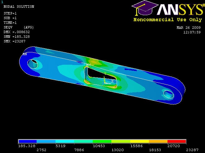
Plot Nodal Solution of von Mises Stress
For a quick refresher on von Mises stress, click Help. Search for von mises and click on the result 2.4 Combined Stresses and Strains (this is lower down among the search results). Read through section 2.4.2.
Main Menu > General Postproc > Plot results > Contour Plot > Nodal Solu
Select Nodal Solution > Stress > von Mises stress and click OK. To change the range of stresses displayed, go to
Utility Menu > PlotCtrls > Style > Contours > Uniform Contours ...
and select User specified. Specify a range of minimum 0 and maximum 25000. We can now see more color variation in the model, and easily pick out the red areas.
When you plot the "Nodal Solution", ANSYS obtains a continuous distribution as follows:
1. It determines the average at each node of the values of all elements connected to the node.
2. Within each element, it linearly interpolates the average nodal values obtained in the previous step.
This procedure is in effect a smoothing operation.
The stress concentration located at the tip of the shaft can be ignored as the force is applied as a point load. Let's look at the results just for the crank by deselecting the elements within the pedal shaft volume. Go to
Utility menu > Select > Entities ...
Select Volumes, By Num/Pick, From Full and click Apply. Pick the crank volume and click OK. After we've selected a volume, we must next select all the elements in this volume. In the Select Entities window, select Elements, Attached to, Volumes and click Apply. Click Replot to display the new selection. Notice the deformation is exaggerated, revealing that deformation is primarily caused by torsion.

To select the whole model again, go to Utility Menu > Select > Everything.
Comparing the σxx Stress with von Mises Stress
To verify that the bending stress in the crank is relatively insignificant, we can compare the element σxx solution with the elemental von Mises solution.
General Postproc > Plot Results > Contour Plot > Element Solu
Click on Stress, then X-Component of stress , then Apply.
If grey areas are appearing in your contour plots, you should go to Utility Menu > PlotCtrls > Style > Contours > Uniform Contours ..., select Auto calculated, and click OK.
Notice that the top-left and bottom-right corners of the cutout area are now blue, and that the scale has been readjusted to show that blue is now a large negative stress value. If this were a case of pure bending, we would expect the top of the crank to be in tension, not compression!
To find out information about specific points on the model, go to
General Postproc > Query Results > Subgrid Solu
Select Stress, X-direction SX, and click OK. The picking window will appear, and you can click on any point in the model. Click OK when finished.

Compare the stress values with the von Mises stress. (Click on von Mises stress, then OK)
Investigate the Stress Concentration
Let's zoom in on the red area. Use the mouse wheel to zoom in and out in the view area. Some other viewing functions: Holding down the Ctrl key and the left mouse button allows you to pan the view, while holding the Ctrl key and the right mouse button allows you to rotate the view. Hold down the right mouse button and draw a rectangle to zoom in on a specific region.
Recall that the nodal solution shows smoothed stress values. Let's compare the nodal solution with the element, i.e. non-smoothed, solution.
General Postproc > Plot Results > Contour Plot > Element Solu
Click on Stress, then von Mises Stress, then the OK button. In the vicinity of the cut-out corners, there are fairly significant discontinuities in the von Mises stress across adjacent elements. This suggests that we need to refine the mesh at least in this region. This is done in the next step.

Calculate Average Strain in Specified Area
In a perfect world, we would be able to validate the ANSYS results by comparing them with strain gage measurements at selected locations. We unfortunately don't have strain gage measurements for this particular geometry but will anyway show you the process by which you can calculate the average strain over an area where a strain gage would be placed. This will help prepare you to compare your ANSYS results with strain gage measurements for a different geometry for which you may have experimental data.
Let's assume that the strain gage is placed on the front face of the crank (z=0.5") roughly halfway between the left hole and the cutout as shown below.

In the coordinate system in our model, let's say this area is given by -1.77"≤ x≤ -1.57" and 0.45"≤ y≤ 0.85". To find the average strain in this area, we will select all nodes that lie in this area and then list the strain values at these nodes. You can copy these values over to Excel or MATLAB to find the average value.
ANSYS provides extensive capabilities, referred to as "select logic", for selecting a subset of the full model using various criteria. We'll use select logic to select the nodes on the front face of the crank. We'll first select the area corresponding to this face.
Utility Menu > Plot > Areas
Utility Menu > Select > Entities
Select Areas from the pull-down menu at the top. Make sure By Num/Pick is selected below that. Click Apply.

Hold down the left mouse button until the front face is picked. Click OK in the pick menu.

Only the area corresponding to this face is selected currently. Verify this by clicking Replot in the Select Entities menu (this replots areas).
One key thing to remember about ANSYS' "select logic" is that the various entity types (areas, volumes, nodes, elements, etc) are selected independently. So all nodes are still "selected", not just the ones that are located on the front face of the crank. Verify this: Utility Menu > Plot > Nodes.
We next select the nodes attached to the previously selected area. In the Select Entities menu, select Nodes from the pull-down menu at the top and Attached to below that. Select Areas, All below that. Click Apply.

Check that only nodes attached to the front face are currently selected by clicking Replot in the Select Entities menu (this replots nodes).
We can get a better idea of where these nodes are located by plotting nodes as well as lines.
Utility Menu > PlotCtrls > Multi-Plot Controls ... > OK
Select Lines and Nodes and click OK.
Utility Menu > Plot > Multi-Plots

From these currently selected nodes, we next select nodes that satisfy the following criterion: -1.77"≤ x≤ -1.57". In the Select Entities menu, retain Nodes at the top. Select By Location and X coordinates below that. Enter Min,Max values as per the snapshot below. Since we want the nodes to be selected from the current set rather than the full set, choose the Reselect radio button. Click Apply and then Replot.

You should see that only the nodes that are in the desired x-coordinate range are selected.

Save your work:Toolbar > SAVE_DB
Next, from the current set of nodes, select nodes that satisfy the following criterion: 0.45"≤ y≤ 0.85" by appropriately modifying the previous select action step. The snapshot below shows what I get: four nodes remain in the selected set. If you mess up, resume from your .db file.

Now all actions on nodes will be performed only on the four nodes that are currently selected. For instance, to list the strain values at these nodes, choose
Main Menu > General Postproc > List results > Nodal Solution > Elastic Strain > X-Component of elastic strain
You can save these values to a text file using File > Save as. You can then read in the values from the text file into Excel or MATLAB for further processing such as finding the average.
Once you are done with the select operations, exit the Select Entities menu and choose
Utility Menu > Select > Everything
Utility Menu > Plot > Nodes
Save your work:Toolbar > SAVE_DB
Go to Step 9: Validate the results
See and rate the complete Learning Module