Numerical Results

Open the Post Processor

In the Project Schematic double click Results to open the post processor. When the A6: Fluid Flow (FLUENT) - CFD - Post Window opens, look at the geometry by clicking the +Z axis on the compass

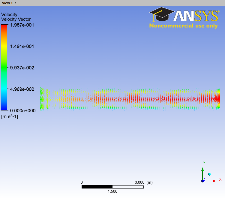
Velocity Vectors

In the Post Processing window, click the Vector icon to create a vector result. When prompted, name the result Velocity Vector. In the Details of Velocity Vector window, begin on the Geometry tab. Under Locations, select Periodic 1. This will show the velocity along the entire geometry surface periodically. Next, click on the Symbol tab. Change the Symbol Size to 0.1. Finally, move to the View tab. We want to see the entire geometry of the pipe: not just half of it like we currently see. To see the whole pipe, check the box next to Apply Reflection/Mirroring, and change the Method to ZX Plane. Because the pipe is long and skinny, it will be difficult to see the results. This post processor allows us to stretch the results to make the results easier to see. To apply a scaling, check the box next to Apply Scale, and change the Scale to 1,10,1 (this will scale the y-direction by 10). When finished, press Apply to see the result. If you wish to see the result without the wireframe of the pipe, uncheck the box next to Wireframe under User Location and Plots.

click here to enlarge

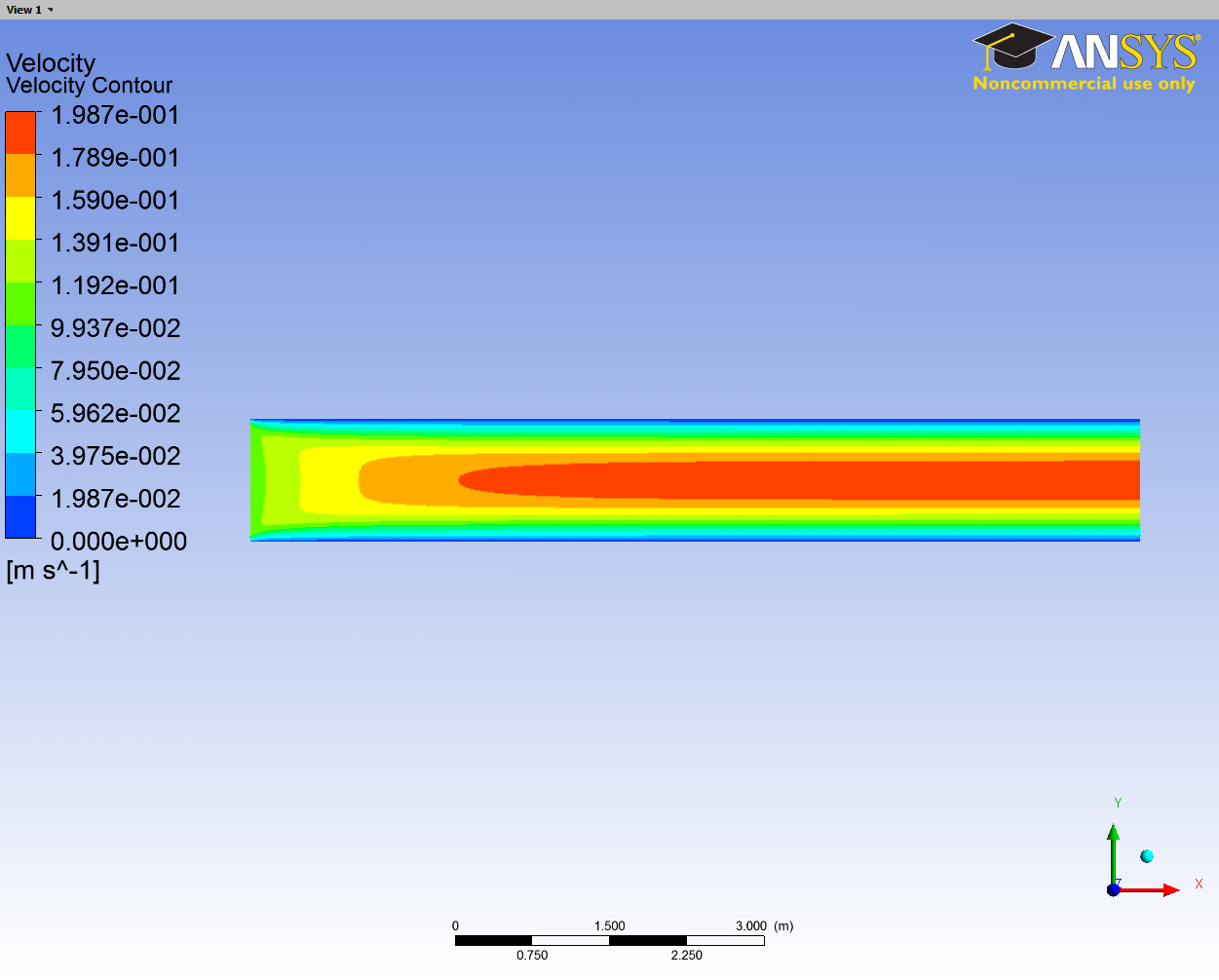
Velocity Contour

In the Post Processing window, click the Contour icon to create a Contour result. When prompted, name the result Velocity Contour. In the Details of Velocity Contour window, begin on the Geometry tab. Under Locations, again select Periodic 1. Also, change the Variable to Velocity. Next, move to the View tab. Check the box next to Apply Reflection/Mirroring, and change the Method to ZX Plane and again,check the box next to Apply Scale, and change the Scale to 1,10,1. When finished, press Apply to see the result. Finally, we need to remove the Velocity Vectors from the Graphic Window. Do this by unchecking the box next to Velocity Vector in the Outline window under User Location and Plots.

Click here to enlarge

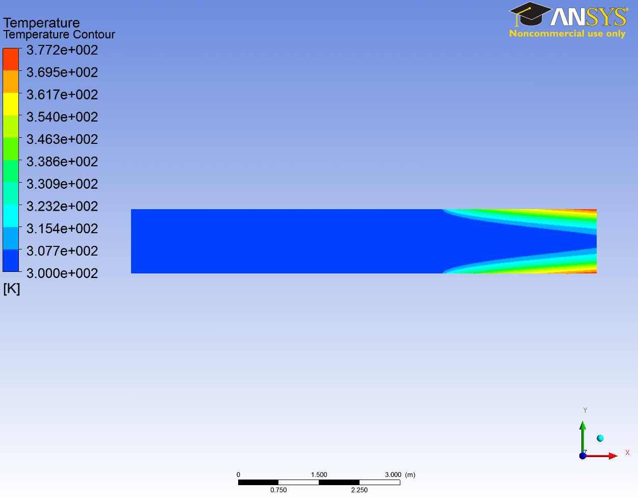
Temperature Contour

In the Post Processing window, click the Contour icon to create another Contour result. When prompted, name the result Temperature Contour. In the Details of Temperature Contour window, begin on the Geometry tab. Under Locations, select Periodic 1. This time, change the Variable to Temperature. Next, move to the View tab. Apply the same mirroring and scaling as we did for the Velocity Contours. When finished, press Apply. Uncheck the box next to Velocity Contour to only see the Temperature Contours.

Click here to enlarge

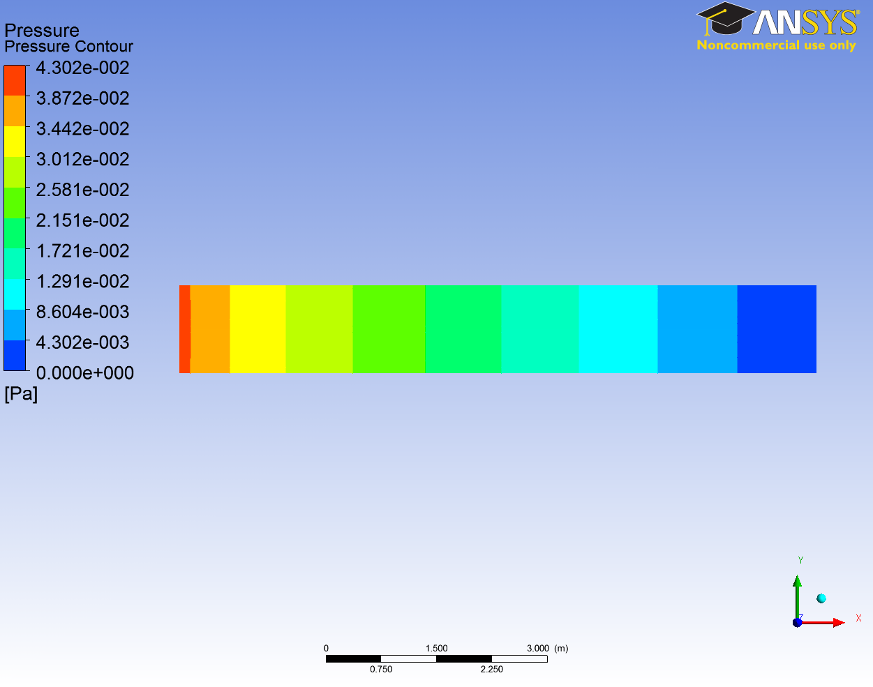
Pressure Contour

Create another contour result, and name Pressure Contour. Use all of the same settings as the previous results but this time choosing Variable > Pressure in the Geometry tab.

Click here to enlarge

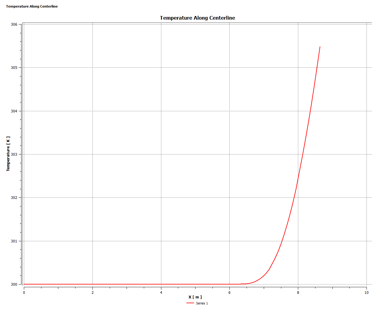
Graph of Temperature along Centerline

To graph the temperature along the centerline, we first need to create the centerline as a path. To accomplish this, click on the Location icon , select Line, and name the line Centerline. In the Details of Centerline window, set the Method to two points. Point 1 is (0,0,0), and Point 2 is (8.64,0,0). Enter these values into the details window. Next, change the number of Samples to 100. Press Apply once finished.

To create a chart, press the chart icon . When prompted, name the page Temperature Along Centerline. In the Details of Temperature Along Centerline window, begin on the General tab. In the Title, enter Temperature Along Centerline. Next, click on the Data Series tab. Under Data Source, in the drop down menu next to Location, select Centerline. Now move to the X Axis tab. In the drop down menu next to Variable, scroll all the way down and select X. In the Y Axis tab, change the Variable to Temperature. when finished, press Apply to see the chart.

Click here to enlarge

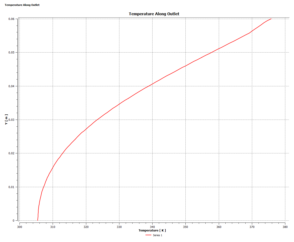
Graph of Temperature along Outlet

To graph the temperature along the outlet, we need to create the outlet as a path much like we did with the centerline. Click on the Location icon , select Line, and name the line Outlet. In the Details of Centerline window, set the Method to two points. Point 1 is (8.64,0,0), and Point 2 is (8.64,0.06,0). Enter these values into the details window. Next, change the number of Samples to 100. Press Apply once finished.

Next, press the chart icon . When prompted, name the page Temperature Along Outlet. In the Details of Temperature Along Outlet window, begin on the General tab. In the Title, enter Temperature Along Outlet. Next, click on the Data Series tab. Under Data Source, in the drop down menu next to Location, select Outlet. Now move to the X Axis tab. In the drop down menu next to Variable, and select Temperature. In the Y Axis tab, change the Variable to Y. when finished, press Apply to see the chart.

Click here to enlarge

Graph of Nusselt Number along the heated section of the pipe

The Nusselt number is a non-dimensional parameter that provides a measure of the convection heat transfer at a surface. It is the ratio of convection to pure conduction heat transfer. We will now derive the Nusselt number as a function of the given parameters and temperature.
The convection heat transfer at the pipe wall is:

We can rearrange terms to find an expression for h, the convection coefficient:

Substitute the convection coefficient expression into the Nusselt Number expression:

where
h is the convection coefficient.
k is the thermal conductivity.
L is the length scale. Similar to the Reynold's Number, the length scale is the diameter of the pipe for an internal pipe flow.
q''_w is the heat flux at the heated surface, 37.5 W/m^2.
Tw is the pipe wall temperature at a given location along the pipe.
Tm is the mean temperature in the pipe at the location where Tw is defined.

Wall Temperature

To find the temperature at the wall, click on insert >> location >> point, and name it Tw exit. In the Details of Tw exit window, set Method to XYZ and enter (8.64, 0.06, 0) in Point.Click Apply to create a point at the upper right corner of the pipe.

Click on Expression right below and right click in the window to create a new expression named Tw. Under Details of Tw panel, enter maxVal(Temperature)@Tw exit in the Definition tab.

Tw now gives the temperature at the location (8.64, 0.06, 0), which is on the exit pipe wall.

Mixed Mean Temperature

To find the mean temperature at a given location in the pipe, click on insert >> location >> line, and name it exit. In the Details of exit window, set Method to Two Points and enter (8.64, 0, 0) for Point 1 and (8.64, 0.06, 0) for Point 2. Click Apply to create a line at the exit of the pipe. The mean temperature is the area weighted average temperature and we can use integral to find the appropriate mean Temperature:

Click on the Calculators tab and double click on Function Calculator. Select lengthInt for the Function, exit for the Location, and Velocity u for the Variable. Check show equivalent expression and click Calculate. The expression "lengthInt(Velocity u)@exit is essentially the integral of u*dr and can be conveniently used to calculate the mean temperature.
Under Expressions, right click in the window to create a new expression and name it Tm. In the Details of Tm window, enter the following:

lengthInt(Velocity u*Y*Temperature)@exit/lengthInt(Velocity u*Y)@exit

This expression will now give the mean temperature at the location in which we called "exit". Recall the pipe radius r is defined in the Y direction in FLUENT. Hence we will use Y to define the radial position in the pipe, as shown in the expression above.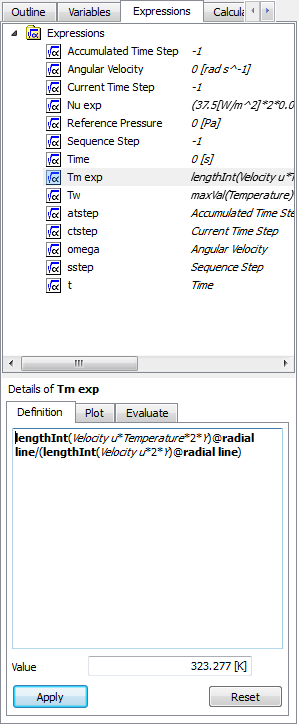

Nusselt Number

We are now ready to find the Nusselt Number. Create another expression and name it Nu exp. Under the Definition tab, enter the Nusselt Number expression shown in the equation above. The units are entered in square brackets, this is done to ensure the expression for the Nusselt Number is dimensionless.

We would like to compare the Nusselt Number along the heated section of the pipe. We can generate the Nusselt Number at a different location by simply changing the x-coordinate of exit and Tw exit, which we defined earlier. Once the new coordinates defined in exit and Tw exit are updated, the associated expression Tw, Tm, and Nu exp will be updated automatically.

We can expect a maximum and dominant convection heat transfer at the entrance of the heated section of the pipe. The convection heat transfer raises the temperature inside the pipe, as well as mean temperature, along the downstream direction. The mean temperature near the exit is higher relative to the entrance and therefore a lower convection heat transfer is expected at the exit. Again, the Nusselt Number is a measure of convection heat transfer relative to conduction heat transfer. Thus we should expect the Nusselt Number to decrease along the length of the pipe.

To export the data, click on the "export" button.  Comma Seperated Value (.csv) is able to be read by matlab and Excel, so it should be fine.

We are now ready to validate and verify our results.

Go to Step 7: Verification & Validation

Go to all FLUENT Learning Modules