ANSYS - 2-D Static Truss

 

Problem Specification
1. Start-up and preliminary set-up
2. Specify element type and constants
3. Specify material properties
4. Specify geometry
5. Mesh geometry
6. Specify boundary conditions
7. Solve!
8. Postprocess the results
9. Validate the results
Problem Set 1
Problem Set 2

This is an introductory tutorial on the ANSYS software package that details how to solve a simple static truss problem. No previous knowledge of ANSYS is assumed in this tutorial.

[Go to Step 0: Problem Specification. ]

Step 2: Specify element type and constants

Enter the Preprocessor module

Main Menu > Preprocessor

This is the module where you create the geometry, specify appropriate displacement constraints and loading, and mesh the geometry. We are more or less going to march down this menu to set up the problem. You will find yourself negotiating through a series of menus as you work off the Main Menu.

Specify Element Type

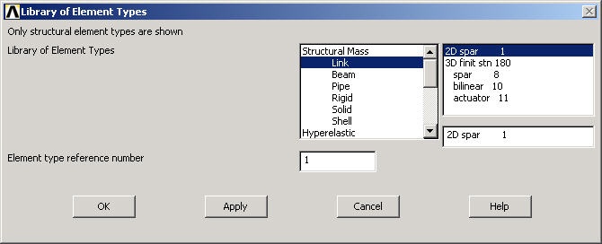
Main Menu > Preprocessor> Element Type > Add/Edit/Delete > Add...

Pick Structural Link in the left field and 2D spar 1 in the right field. Click OK to select this element.

Now you will see the following in the Element Types dialog box:

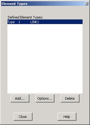
LINK1 appears as the only defined element type in the Element Types dialog box. To view the help pages for this element type, click on Help in the Element Types dialog box. This brings up the Help window. Click on Search in the left pane and type in LINK1. (If the left pane is hidden, click the Show button in the toolbar) The first search result is the help page for the LINK1 element. Note that this is a two-dimensional spar element that supports uniaxial tension and compression but not bending, so it is appropriate for modeling a truss structure. There are two degrees of freedom at each of its two nodes: translations in the nodal x and y directions. The "1" in the element name is the internal reference number for this element type in ANSYS' list of available element types.

Before proceeding, let's take a quick peek at the pictorial summary of the element types available in ANSYS. Click on Release 10.0 Documentation for ANSYS > Element Reference > Element Characteristics > Pictorial Summary in the left part of the Help window. Our own humble LINK1 element is listed at the top of the pictorial summary. Clicking on the LINK1 box will take you to the help page for the element that we just visited. In general, you need to take the time to understand the element types and pick the appropriate one(s) for your problem. The pictorial summary is a good place to start for identifying the appropriate element for your problem. Your choice of element type has a significant effect on the speed and accuracy of the solution.

Minimize the Help window.

Close the Element Types window by clicking Close.

Specify Element Constants

Main Menu > Preprocessor > Real Constants > Add/ Edit/ Delete

This opens up the Real Constants dialog box. Click Add.... This brings up the Element Type for Real Constants dialog box with a list of the element types defined in the previous step. We have only one element type, LINK1, defined and it's automatically selected. Click OK.

We now enter the constants needed for the LINK1 element. For AREA, enter 0.01 which is the cross-sectional area of the element. We'll work in SI units. Leave the Initial strain field blank since it's not applicable to our problem.

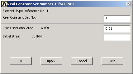
It is the responsibility of the ANSYS user to make sure that the values entered are in consistent units. Click OK.

We see in the Real Constants menu that the constant set that we just created is "Set 1". So, when we mesh the geometry later on, we'll use the reference no. 1 to assign this constant set.

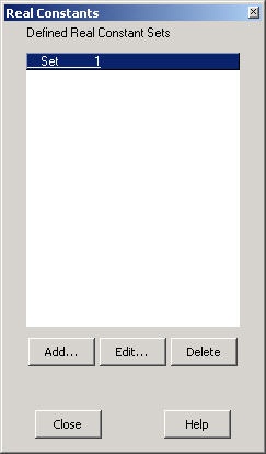
Click Close in the Real Constants dialog box.

Step 3: Specify material properties

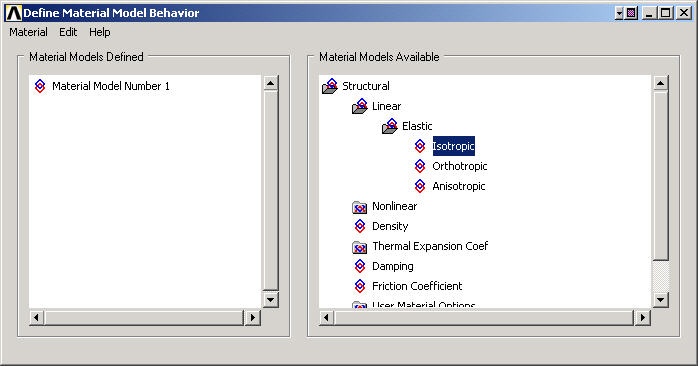
Main Menu > Preprocessor > Material Props > Material Models

In the Material Models Available Frame of the Define Material Model Behavior window, double-click on Structural, Linear, Elastic_, and_ Isotropic.

Enter 200e9 for Young's Modulus EX.
Enter 0.3 for Poisson's Ratio PRXY.

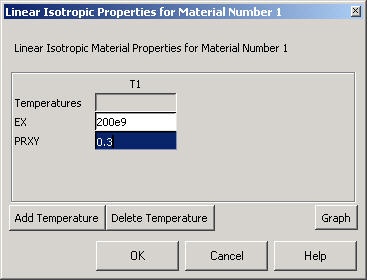
Click OK. This completes the specification of Material Model Number 1. When we mesh the geometry later on, we'll use the reference no. 1 to assign this material model. Close the Define Material Model Behavior menu.

Save your work

Utility Menu > File > Save as Jobname. db

This saves all the relevant data into one file called truss. db in your working directory, truss being taken from the jobname and db being an abbreviation for database. Verify that ANSYS has created this "database file" in your working directory. You can restart from your last save at any time using Utility Menu > File > Resume Jobname. db or ANSYS Toolbar > RESUM_DB. Each time you successfully finish a series of steps, you should save your work. Unfortunately, ANSYS doesn't have an undo button (though that is the first thing I needed while learning ANSYS!) and one way to recover from mistakes is to resume from your last save.

Step 4: Specify geometry

Overview

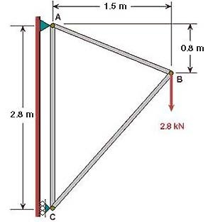
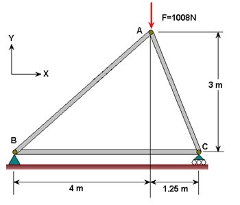
Since we are using the 2D Spar element, we can represent each truss member by a line. A line can be created by joining two keypoints (ANSYS terminology for vertices). So we'll need three keypoints, located at A, B and C in the figure below. We'll locate the origin of the coordinate system at C and number the keypoints at A, B and C as 1, 2 and 3, respectively.

Create Keypoints

Main Menu > Preprocessor > Modeling > Create > Keypoints > In Active CS

The active CS (i.e. Coordinate System) is the global Cartesian system by default and we'll work only in this coordinate system in our friendly introduction. ANSYS offers the capability to switch between various types of coordinate systems which will be necessary when you move on to solving super-duper problems.

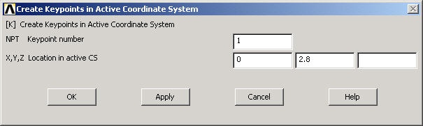
In the Create Keypoints in Active Coordinate System dialog box,

Enter 1 for Keypoint number
Enter 0 for X and 2.8 for Y
(The Z value defaults to zero)
Click Apply (which accepts the input and then brings back the dialog box for further input)

Note that you can move to the next field using the Tab key.

Enter 2 for Keypoint number
Enter 1.5 for X and 2.0 for Y
Click Apply

Enter 3 for Keypoint number
Enter 0 for X and 0 for Y
Click OK (which accepts the input and then closes the dialog box)

Note the difference between Apply and OK which holds throughout ANSYS.

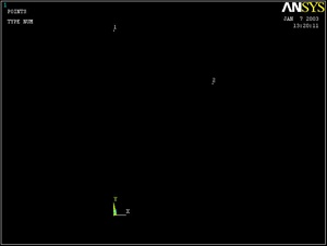
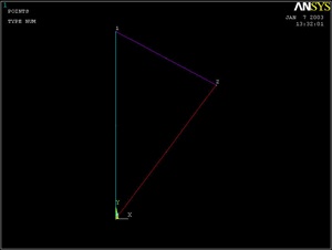
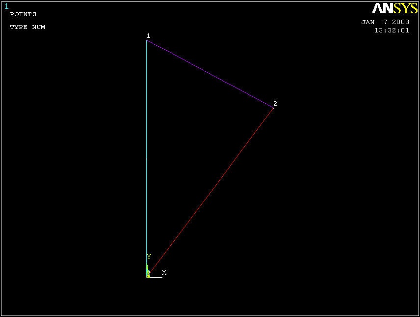
The keypoints will now be displayed in the Graphics window along with a triad that indicates the origin of the coordinate system (coincident with keypoint 3 in our case) and the axes.

fluent:See larger version

Check Keypoints

To check if the keypoints have been created correctly:

Utility Menu > List > Keypoints > Coordinates only

This brings up a window listing the coordinates and rotation angles for the keypoints. Verify that you have the following:

 

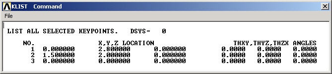
You can rotate the coordinate system associated with each keypoint and that is what the rotation angles THXY, THYZ and THZX refer to. In our case, we don't need to rotate the keypoint coordinate system and so the rotation angles are identically zero.

Close the window listing the keypoints.

Close the Keypoints and Create menus.

Modifying Keypoints (If Necessary)

If you are like me, you made a mistake while creating keypoints and cursed that there is no undo button. To correct your mistake(s), you can delete keypoints and re-create them. In case you need to delete a keypoint, do the following:

Main Menu > Preprocessor > Modeling >Delete > Keypoints

This brings up the so-called pick menu.

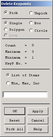
Click on the keypoint you want to delete. A square appears around that keypoint indicating that it is selected. (Repeat for other keypoints as necessary.)
Click OK in the pick menu.

You should see the keypoint disappear in the Graphics window. You can also check that the keypoint has been deleted using Utility Menu > List > Keypoints. You can then re-create the keypoint.

Save your work

Once you have successfully created the keypoints, save your work using

Toolbar > SAVE_DB

This is a short-cut for

Utility Menu > File > Save as Jobname. db

Create Lines from Keypoints

Main Menu > Preprocessor > Modeling > Create > Lines > Lines >In Active Coord

This will bring up the Lines in Active Coord pick menu.

To create the line between keypoints 1 and 3, click on keypoint 1 and then keypoint 3. Similarly, create lines between keypoints 1 & 2 and keypoints 2 & 3.

fluent:See larger version

Close the Lines in Active Coord pick menu by clicking on Cancel.

Close the Lines and Create menus.

Check Lines

Take a look at the list of lines that have been created:

Utility Menu > List > Lines

Click OK to accept the default output format.

The first four columns in the list should be:

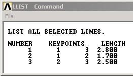
The order of the keypoints for a line doesn't matter i.e. line l1 could go from keypoint k1 to k2 or equivalently, k2 to k1.

Close the window listing lines.

Modifying Lines (If Necessary)

If a line doesn't look right, you can delete and re-create it. To delete a line:

Main Menu > Preprocessor > Modeling > Delete > Lines Only

This brings up the pick menu.

Click on the line you want to delete in the Graphics window. Click OK. This deletes the line.

Save your work

Once you have successfully created the lines, click on Toolbar > SAVE_DB to save the database.

Step 5: Mesh geometry

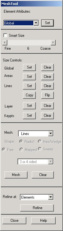
Each truss member can be represented as a 2D Spar element. We'll use the MeshTool to mesh the geometry with this element.

To bring up the MeshTool, select

Main Menu > Preprocessor > Meshing > MeshTool

The MeshTool is used to control and generate the mesh.

Set Meshing Parameters

We'll now specify the element type, real constant set and material property set to be used in the meshing. Since we have only one of each, we can assign them to the entire geometry using the Global option under Element Attributes.

Make sure Global is selected under Element Attributes and click on Set.

This brings up the Meshing Attributes menu. You will see that the correct element type, material number and real constant set are already selected since we have only one of each.

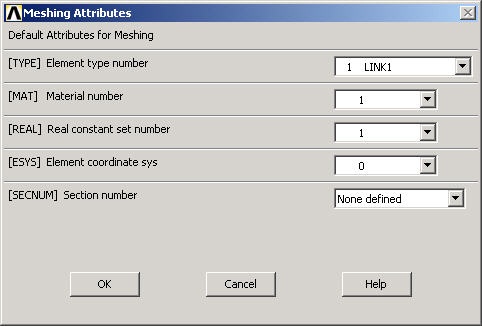
Click OK. ANSYS now knows what element type (and associated constants) and material type to use for the mesh.

Set Mesh Size

Since a LINK1 element is equivalent to a truss member, we will specify that we want only one element per line. This is a subtle point and also very unusual; in most problems, you want to subdivide your part into many elements.

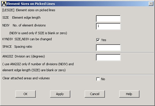
In the MeshTool, under Size Controls and Lines , click Set.

In the pick menu that comes up, click Pick All (since we want the specification of mesh size to apply to all lines in the geometry). This brings up the Element Sizes on Picked Lines menu. Specify No. of element divisions to be 1. Click OK*.* ANSYS will now use 1 element to mesh each line.

Mesh Lines

In the MeshTool, make sure Lines is selected in the drop-down list next to Mesh. This means the geometry components to be meshed are lines (as opposed to areas or volumes, as we'll see later). Click on the Mesh button.

This brings up the pick menu. Since we want to mesh all lines, click on Pick All. The lines have been meshed. This is reported in the Output Window (usually hiding behind the Graphics Window):

NUMBER OF LINES MESHED = 3
MAXIMUM NODE NUMBER = 3
MAXIMUM ELEMENT NUMBER = 3

Close the MeshTool.

View Element List

Utility Menu > List > Elements > Nodes + Attributes

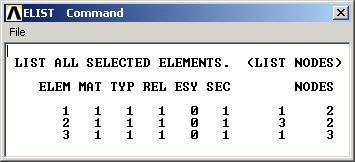
This table says that Element 1 is of material type 1 and element type 1 and is attached to nodes 1 and 2 and so on. In this element list, the order of the two nodes for each element doesn't matter. For example, element 3 can be attached to nodes 2 and 3 or equivalently, nodes 3 and 2. Also, the order of element numbering is not important since it is for internal bookkeeping.

Close the window listing the elements.

View Node Location

In order to see where the nodes are located, you can look at the list of nodes.

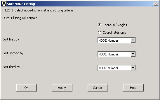
Utility Menu > List > Nodes

In Sort NODE Listing menu, click OK to accept defaults.

My list of nodes looks like this:

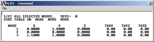
From the node and element lists, one can conclude that in this case:

Node 1 is pin A
Node 2 is pin C
Node 3 is pin B

Element 1 is member AC
Element 2 is member AB
Element 3 is member BC

Your own node and element numbering might be different from this and you would have to account for this while interpreting results in the postprocessing step.

Close the window listing the nodes.

Save your work

Toolbar > SAVE_DB

Step 6: Specify boundary conditions

Next, we step up to the plate to define the boundary conditions, namely, the displacement constraints and loads. Note that in ANSYS terminology, the displacement constraints are also "loads". We can apply the loads either to the geometry model or to the finite-element model (that is to the elements and nodes directly). The advantage of the former is that one doesn't have to re-specify the constraints on changing the mesh. So we'll apply the constraints to the geometry i.e. to the keypoints.

You can see from the diagram that the pin at A is constrained in x and y directions; or equivalently, keypoint 1 is constrained such that its UX and UY displacements are zero. Similarly, keypoint 3 is constrained such that its UX displacement is zero.

Apply Displacement Constraints

Main Menu > Preprocessor > Loads > Define Loads > Apply > Structural > Displacement > On Keypoints

This brings up the Apply U, ROT on KPs pick menu.

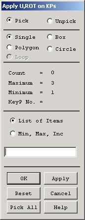
In the Graphics window, click on keypoint 1;
This will draw a small square around keypoint 1 to indicate that it's been picked.

In the pick menu, click Apply_._ The following menu shows up.

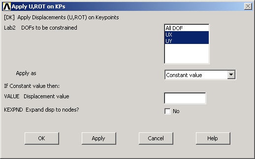
Since we want to constrain UX as well as UY to zero at keypoint 1, select both UX and UY from items in DOFs to be constrained list. Since the Displacement value is zero by default, leave that field empty. Click on Apply.

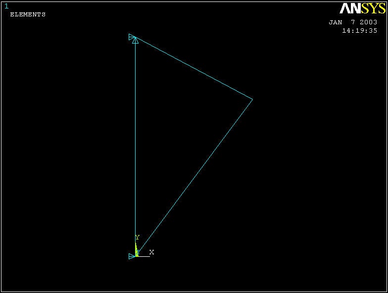
You will see triangle symbols appear in the Graphics window indicating that both UX and UY DOFs are constrained at keypoint 1.

Next we apply the displacement constraint at keypoint 3. In the Graphics window, click on keypoint 3. In the pick menu, click Apply. Select only UX from items in DOFs to be constrained list. Click OK.

You will see a triangle symbol appear indicating that only the UX DOF is constrained at keypoint 3.

Close the Displacement and Apply menus.

List Displacement Constraints

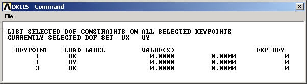
You can verify the displacement constraints on the model by listing them.

Utility Menu > List > Loads > DOF constraints > On All Keypoints

This brings up a window with the constraint information.

If you made a mistake in applying a constraint, you can delete and reapply it. You can delete a constraint using Main Menu > Preprocessor > Loads > Define Loads >Delete > Structural > Displacement > On Keypoints. Alternately, you can resume from your last save and continue from there.

Close the window listing the constraint information.

Save the database: Toolbar > SAVE_DB

Apply Loading

We have only one load to apply on the structure, namely, the 2800 N force in the negative y-direction at keypoint 2 (see figure 1).

Main Menu > Preprocessor > Loads > Define Loads > Apply > Structural >Force/Moment > On Keypoints

This brings up the Apply F/M on KPs pick menu.

In the Graphics window, click on keypoint 2; then in the pick menu, click OK.

In the menu that appears, select FY for Direction of force/ mom.

Enter -2800 for Force/ moment value. Click OK.

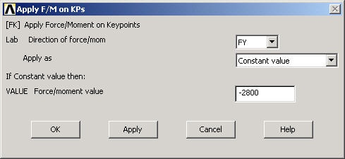
The negative sign for the force indicates that it is in the negative y-direction. You'll see a vector indicating the applied force in the Graphics window.

Close the Force/ Moment, Apply, Loads and Preprocessor menus.

Save the database: Toolbar > SAVE_DB

Step 7: Solve!

Enter Solution Module

Main Menu > Solution > Solve > Current LS

This solves the current load step (LS) i. e. the current loading conditions. In our problem, there is only one load step; ANSYS allows for multiple load steps that can be solved sequentially without leaving the Solution module.

Review the Problem

Review the information in the /STAT Command window. This is a summary of the problem that ANSYS is about to solve.

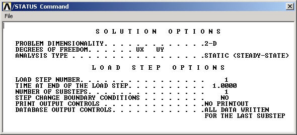
Close this window.

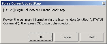
Perform Solution

Click OK in Solve Current Load Step menu.

ANSYS performs the solution and a yellow window should pop up saying "Solution is done!". Congratulations! You just obtained your first ANSYS solution.

Close the yellow window.

In preparation for the postprocessing step to be undertaken next, exit the solution module by closing the Solution menu.

Verify that ANSYS has created a file called truss.rst in your working directory. This file contains the results of the (previous) solve. The rst extension in the filename stands for results from a structural analysis. The truss.db file contains only steps 1-6. To resume your work subsequent to exiting ANSYS, you'll have to first resume from the jobname.db file and then read in the results from the jobname.rst file using

Main Menu > General Postproc > Read Results > First Set

This is one of the many ANSYS quirks you'll encounter as you work with the program.

Step 8: Postprocess the results

Postprocessing is the step where we look at and analyze the results obtained from the ANSYS solution.

Enter the General Postprocessing module_:_

Main Menu > General Postproc

Plot Deformed Shape

Main Menu > General Postproc > Plot Results > Deformed Shape

Select Def + undeformed and click OK.

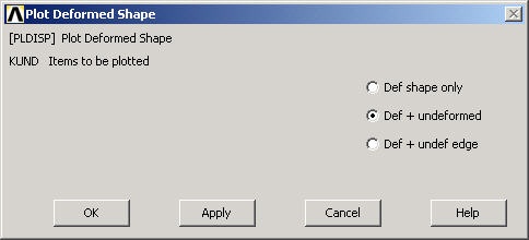
This plots the deformed and undeformed shapes in the Graphics window.

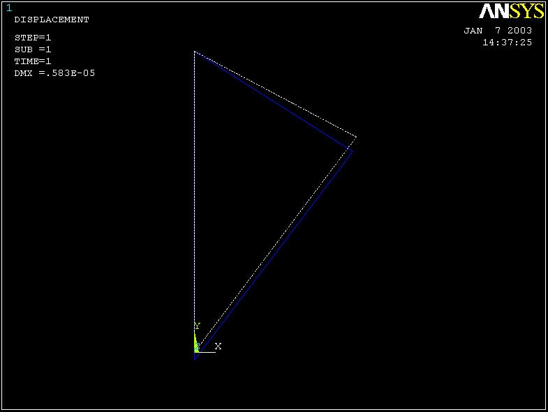
The deformed shape is shown as a solid line and the undeformed shape as a dotted line. The maximum displacement DMX is 0.583E-05m as reported in the Graphics window. This is small but plausible. Note that the deformation is magnified in the plot so as to be easily visible.

To save the deformation plot in a file, use Utility Menu > PlotCtrls > Hard Copy > To File. Select the file format you want and type in a filename of your choice under Save to: and click OK. The file will be created in your working directory. You can print out this file as necessary.

Animate the deformation:

Utility Menu > PlotCtrls > Animate > Deformed Shape

Select Def + undeformed and click OK. Select Forward Only in the Animation Controller.

Node 1 (Pin A) doesn't move and node 2 (Pin C) moves only in the vertical direction. Node 3 (Pin B) moves more or less in the direction of the applied force. The deformation of the structure agrees with the applied boundary conditions and matches with what one would expect from intuition.

Turn On Node and Element Numbers

In order to interpret the results that ANSYS reports, it's useful to turn on the node and element numbers in the Graphics window.

Utility Menu > PlotCtrls > Numbering

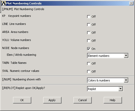
The Plot Numbering Controls menu is used to control the numbering of the various entities in a finite-element model.

Turn on Node numbers. Under Elem/Attrib numbering, select Element numbers. Click OK.

The node and element numbers will now appear in the Graphics window.

List Forces in Truss Members: Method 1

Main Menu > General Postproc > List Results > Element Solution

From the list, under Element Solution, select All Available force items . Click OK.

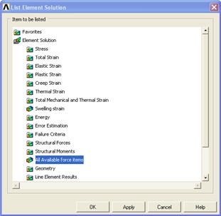
This brings up a window listing the forces that the elements apply on each of their nodes:

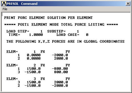
These element forces reported by ANSYS are forces ON its environment BY the element, not the converse. For example, Element 2 (or member AB) applies a force of 1500 N in the x-direction and 800 N in the negative y-direction on node 1 (or pin A). This means that the total force in AB is . The resultant acts from A to B i.e. the member is pulling on pin A. So it must be in tension. Similarly, the force in Element 1 (AC) is 2000 N (tension) and in Element 3 (BC) is 2500 N (compression). Note that your node and element numbers might be different from the above since they depend on the order in which the lines were created.

Close the PRESOL Command window.

List Forces in Truss Members: Method 2

Bring up the help page for LINK1 element:

Utility Menu > Help > Help Topics

Under the Contents tab, select

Release 10.0 Documentation for ANSYS > Element Reference > Element Library > LINK1

In the LINK1 help page, scroll down to LINK1 Element Output Definitions. You'll see the item

MFORX: Member force in the element coordinate system X direction

The figure at the top of the LINK1 help page shows that the x-direction in the element coordinate system is along the line. So MFORX is basically the axial force in the element.

So how do we get the MFORX values for our three elements from ANSYS? ANSYS has a quirky way of doing this as we shall see. If you scroll down the help page further, you'll see the LINK1 Item and Sequence Numbers:

MFORX SMISC 1

The output data is broken down into item groups with SMISC being one of the groups. Each item within an item group has an identifying "sequence" number. So MFORX is the item with sequence number 1 in the SMISC group.

Minimize the help window. To list MFORX values:

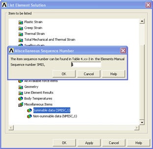
Main Menu > General Postproc > List Results > Element Solution

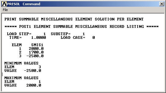
Under Element Solution, select Miscellaneous Items > Summable data (SMISC,1). Since MFORX is sequence number 1 in the SMISC group, enter 1 next to Sequent number SMIS in the editable field. Click OK. Click OK in the List Element Solution window.

This brings up a window with the axial forces in the elements. Positive values indicate tension and negative values compression. Do these values match what we got in method 1?

You can also plot the items listed under Element Output Definitions using the sequence number.

In most cases, you plot stresses using Main menu > General Postproc > Plot Results > Contour Plot >Nodal Solu. But for line elements like LINK1, this doesn't work and you'll get zero values for the stresses. So you'll have to use the sequence numbers to make stress plots for line elements.

List Reaction Forces at Nodes

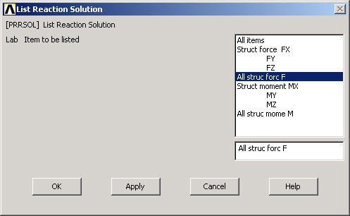
Main Menu > General Postproc > List Results > Reaction Solu

Select All struc forc F for Item to be listed and click OK.

This brings up a window with the reaction forces at the nodes.

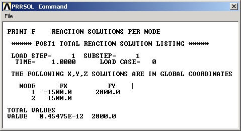
The sum of the reaction forces balances the applied load as should be the case for static equilibrium.

Close the PRRSOL Command window.

Step 9: Validate the results

Do not assume that if you are able to obtain a solution from ANSYS, it is bound to be correct. It is very important that you take the time to check the validity of your solution. This section leads you through some of the steps you can take to validate your solution.

Simple Checks

• Does the deformed shape look reasonable and agree with the applied boundary conditions? We checked this in step 8.
• Do the reactions at the supports balance the applied forces for static equilibrium? We checked this also in step 8.

Refine Mesh

The results obtained from FEA analysis depend on the mesh. An important step in the analysis is to make sure that the mesh resolution is adequate for the desired level of accuracy. This is done by refining the mesh and comparing results obtained with different levels of mesh resolution.

In our truss example, however, a truss member has to be modeled as a single LINK1 element. If we use multiple LINK1 elements to model a single truss member, these elements can rotate freely with respect to each other since they are essentially linked through pin joints. This violates physical reality and is one of the few cases where we'll avoid refining the mesh since it leads to an incorrect result.

Compare with Theory

Results should be compared with appropriate theoretical results whenever possible. In most cases, one would use theory to obtain order-of-magnitude estimates rather than to make a head-to-head comparison since presumably FEA is being used because a theoretical solution is not available. In this case, however, one can easily determine the forces in the truss members using the method of joints from statics. I'd recommend that you take a few minutes during commercials on your favorite TV show to calculate the forces and compare them with your ANSYS results.

Exit ANSYS

Utility Menu > File > Exit

Select Save Everything and click OK.

This is just a quick introduction to ANSYS to give you a flavor of what a full-fledged engineering package looks like. If it felt unfriendly or cumbersome, you are not alone; I went through this myself (otherwise, congratulations! you are a genius). It takes some getting used to. Believe it or not, it gets a lot easier to use with time. You have a lot of years ahead of you to gain the experience necessary to harness the power of finite-element analysis. All the ANSYS features including the underlying theory are documented online and can be accessed using Utility Menu > Help. There are tutorials available in the documentation which are also useful.

Problem Set 1

Consider the case where the displacement constraints at A and C are interchanged i.e.

• at A, only UX is set to zero
• at C, both UX and UY are set to zero

1. How would you expect the reaction forces at the supports A and C to change?

2. What can you say about how the x-component of the forces in the truss will change?

Re-solve the truss problem with the modified constraints. Fom your ANSYS solution:
1. List the reactions. Note that you can save the reaction listing as follows: in the window that comes up with the listing of the reaction forces, click on:

File > Save As

2. Determine the force in each truss member and whether the member is in tension or compression.

Tips: Start from your ANSYS solution to the truss tutorial problem but use a different job name as follows:

• Start the ANSYS Product Launcher. Specify the same directory as for the tutorial but use a different jobname. Once ANSYS comes up, select: Utility Menu > File > Resume from. Choose truss.db and click OK.

Note that you can delete constraints using:

Main Menu > Preprocessor > Loads > Define Loads > Delete

It works similar to how you apply loads.

You can plot the displacement constraints in the Graphics window as follows:

Utility Menu > Pltctrls > Symbols

Select All Applied BCs for Boundary condition symbol. Click OK.

You might have to use :

Utility Menu > Plot > Replot

or

Utility Menu > Plot > Multi-plots

for the constraint symbols to appear in your plot.
Go to Problem Set 2

See and rate the complete Learning Module

Go to all ANSYS Learning Modules

Problem Set 2

Determine the force in each member of the following truss using ANSYS. Indicate if the member is in tension or compression. Use the same LINK1 element as in the tutorial. The cross-sectional area of each member is 0.02 m², Young's modulus is 200x10⁹ N/m² and Poisson's ratio is 0.3. Verify your results by calculating the forces manually.

Results

Determine the following:

1. Listing of the reactions from the ANSYS solution.

2. Listing of the element forces from the ANSYS solution. Calculate and determine the forces in each member and whether the member is in tension or compression from this ANSYS result.

3. Using your pencil-and-paper calculations verifying the ANSYS results for the member and reaction forces.

See and rate the complete Learning Module

Go to all ANSYS Learning Modules