 Sign-up for free online course on ANSYS simulations!
Unknown macro: {rate}
Author: Rajesh Bhaskaran, Cornell University
Problem Specification
1. Start-up and preliminary set-up
2. Specify element type and constants
3. Specify material properties
4. Specify geometry
5. Mesh geometry
6. Specify boundary conditions
7. Solve!
8. Postprocess the results
9. Validate the results
Note Title
The following ANSYS tutorial is under construction.
Problem Specification
A preeminent bicycle company is disappointed with the negative feedback they have received on their latest model, and they have pinpointed the problem to an outdated bicycle crank design that they assumed would still withstand typical loads. To protect their reputation, they have outsourced the task of analyzing the crank to you, providing you with the geometry of the bicycle crank and attached pedal shaft shown below. The dimensions are given in inches. The material they selected has an Young's modulus E=2.8x10⁷ psi and Poisson ratio ν=0.3.

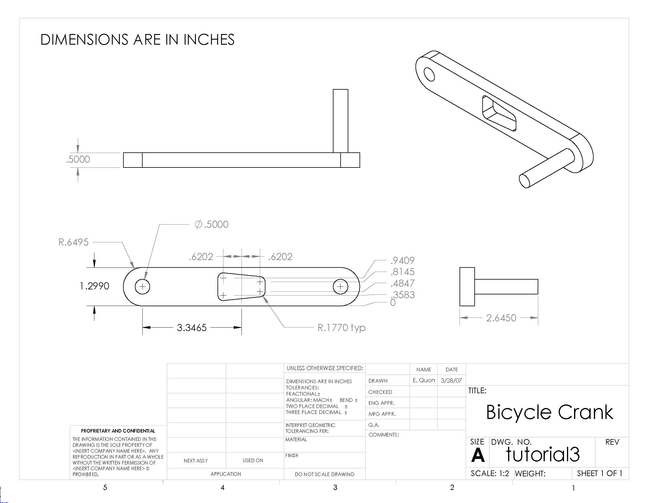
Using ANSYS, determine the mechanical response due to a load of 100 lbf applied vertically downward at the end of the pedal shaft as shown in the figure below. Assume that the crank is attached rigidly to a fixed shaft fitted into the hole near the left end of the crank. This means you can constrain the surface of the left hole in X, Y and Z directions as indicated below.

Calculate the deflection, strain and stress distributions in the crank/pedal shaft combination for this loading condition. Use the ANSYS results to evaluate the degree of stress concentration in the vicinity of the cut-out in the crank geometry.
Go to Step 1: Start-up and preliminary set-up
See and rate the complete Learning Module
Go to all ANSYS Learning Modules
Step 1: Start-up and preliminary set-up
Start ANSYS
Create a folder called crank at a convenient location. We'll use this folder to store files created during the ANSYS session.
Start > All Programs > ANSYS 12.0 > Mechanical APDL Product Launcher
In the window that comes up, enter the location of the folder you just created as your Working Directory by browsing to it. All files generated during the ANSYS run will be stored in this directory.
Specify crank as your Job Name. The job name is the prefix used for all files generated during the ANSYS session. For example, when you perform a save operation in ANSYS, it'll store your work in a file called crank.db in your working directory.
For this tutorial, we'll use the default values for the other fields. Click Run. This brings up the ANSYS interface. To make best use of screen real estate, move the windows around and resize them so that you approximate this screen arrangement. This way you can read instructions in the browser window and implement them in ANSYS. Note that this tutorial has been formatted to fit in a skinny browser window. If your monitor screen is small, you can use Alt+Tab keys to conveniently switch between the ANSYS and browser windows (this trick works in Microsoft Windows).
You can resize the text in the browser window to your taste and comfort:
In Internet Explorer, select Menubar > View > Text Size, then choose the appropriate font size.
In Mozilla Firefox, select Menubar > View > Zoom.
Set Preferences
As before, we'll more or less work our way down the Main Menu.
Main Menu > Preferences
In the Preferences for GUI Filtering dialog box, click on the box next to Structural so that a tick mark appears in the box. Click OK.

Recall that this is an optional step that customizes the graphical user interface so that only menu options valid for structural problems are made available during the ANSYS session.
Go to Step 2: Specify element type and constants
See and rate the complete Learning Module
Go to all ANSYS Learning Modules
Step 2: Specify element type and constants
Specify Element Type
We next select the appropriate element type(s) for our problem from a large list of about 200 candidates. Consider this as equivalent to rifling through a sizable toolchest, picking out one or more tools and placing them on a table for later use (in step 5, in our case). To see which element types are appropriate for this problem, bring up the pictorial summary of element types: Utility menu > Help > Help Topics. Search for "pictorial summary" and double-click on the search result titled 3.2 Pictorial Summary. Click on the link to SOLID Elements. These are the element types you can use to mesh a solid volume. Check out the Solid45 element type. It is a brick-shaped element of the type referred to as "hexahedral" or "hex". It has a node at each corner and each node has three degrees of freedom: displacement in the x, y and z directions.

Click on the SOLID45 link in the pictorial summary. This takes you to the help page for this element. Read through the juicy information at the beginning of this help page. Note that there are no real constants to be defined in our case. Click on SOLID45 in the statement "See SOLID45 in the Theory Reference for ANSYS and ANSYS Workbench for more details about this element" which appears near the top of the help page. Click on Equation 12-188. This shows you the shape function for the element i.e. the equation used to determine the displacement at a general point within the element from the displacement values at the 8 nodes.
We will create our volume mesh in two steps:
- Mesh the front surfaces of the crank as well as the pedal shaft.
- Extrude these surface meshes to get the corresponding volume meshes.
This is analogous to creating a sketch and then extruding while making a solid in a CAD package. Since we cannot mesh surfaces with SOLID45, we need an additional element type called MESH200. Go back to the pictorial summary of element types. Scroll to the top of the page and click on the link to MESH Elements. This takes you to the MESH200 element type.

Click on the MESH200 link in the pictorial summary to see the help page for this element. You see the following information:
"MESH200 is a "mesh-only" element, contributing nothing to the solution. This element can be used for the following types of operations:
- Multistep meshing operations, such as extrusion, that require a lower dimensionality mesh be used for the creation of a higher dimensionality mesh"
In our case, meshing the two front surfaces with MESH200 elements can be thought as going to these surfaces and marking out points and lines with a pen to show ANSYS where to put the corresponding SOLID45 nodes and element faces. The SOLID45 nodes and elements are actually placed at these pre-marked locations in the extrusion step. In effect, MESH200 provides greater control over the mesh without actually contributing to the solution.
Referring to Figure 200.1 in the MESH200 help page, we see that this element type comes in 12 different flavors. For our purposes, we will be using the 3-D quadrilateral with 4 nodes option since this corresponds to an element face of SOLID45. The help page indicates that this option is selected by setting KEYOPT(1) = 6. Note that there are no real constants to be defined for MESH200.
Minimize the ANSYS Help window. Select
Main Menu > Preprocessor> Element Type > Add/Edit/Delete > Add...
Pick Structural Mass Solid in the left field and Brick 8node 45 in the right field. Click Apply to select this element.

Scroll down the left field, pick Not Solved in this field and then Mesh Facet 200 in the right field. Click OK to select this element.

The Element Types window should list two types of elements: MESH200 and SOLID45.

In order to set the 3-D quadrilateral with 4 nodes option for MESH200, click on MESH200 and then Options ... in the above menu. Then, select QUAD 4-NODE next to Element shape and # of nodes K1. Click OK.

Close the Element Types menu.
Specify Element Constants
There are no real constants to be set for either element type as noted above.
Save your work
Toolbar > SAVE_DB
Go to Step 3: Specify material properties
See and rate the complete Learning Module
Go to all ANSYS Learning Modules
Step 3: Specify material properties
Main Menu > Preprocessor >Material Props > Material Models
In the Define Material Model Behavior menu, double-click on Structural, Linear, Elastic, and Isotropic.

Enter 2.8E7 for Young's modulus EX, 0.3 for Poisson's Ratio PRXY. Click OK.

To double-check the material property values, double-click on Linear Isotropic under Material Model Number 1 in the Define Material Model Behavior menu. This will show you the current values for EX and PRXY. Cancel the Linear Isotropic Properties window.
This completes the specification of Material Model Number 1. When we mesh the geometry later on, we'll use the reference no. 1 to assign this material model. Close the Define Material Model Behavior menu.
Save your work
Toolbar > SAVE_DB
Go to Step 4: Specify geometry
See and rate the complete Learning Module
Go to all ANSYS Learning Modules
Step 4: Specify geometry
Note that you can import geometry from a CAD package such as Pro/Engineer or SolidWorks into ANSYS by following these instructions.
Since the geometry excluding the cutout region is symmetric with respect to the vertical centerline, we will model half of the crank and then mirror the other half to complete the crank body. Then we will create the cutout from a set of keypoints.
Create a Rectangular Area
Main Menu > Preprocessor > Modeling > Create > Areas > Rectangle > By 2 Corners
Enter the values as shown below. Click OK.

It may be helpful to turn on area numbering to identify the different areas you create.
Utility menu > PlotCtrls > Numbering ...
Check the box next to AREA Area numbers to turn on area numbering. Click OK.

Create Circular Areas
Main Menu > Preprocessor > Modeling > Create > Areas > Circle > Solid Circle
Enter the values as shown below. Click Apply. This creates the rounded end of the crank.

Enter the new set of values shown below. Click OK. This creates the area for a hole.

Your window should look something like the picture below. You can click Utility Menu > Plot > Replot or click on the Fit View  button on the right toolbar to refresh the view.

To correct any mistakes, you must click Main Menu > Preprocessor > Modeling > Delete > Areas Only and then pick each area you want to remove. The mouse pointer will show an up arrow for picking areas and a down arrow for un-picking areas. Right-click to switch between pick and unpick mode. When you have made all your selections, click OK. Click Utility Menu > Plot > Replot to refresh the view.
Add Areas
Main Menu > Preprocessor > Modeling > Operate > Booleans > Add > Areas
Pick the rectangular and large circular areas. Click OK. (This is where the area numbering may come in handy) The result should look like the image below.

Subtract Hole Area
Now we create the hole by subtracting the round area from the rest of the crank.
Main Menu > Preprocessor > Modeling > Operate > Booleans > Subtract > Areas
First pick the body of the crank and click OK. Then pick the hole, and click OK again. The result is shown below.

Reflecting the Area
To create the other half of the crank, we will reflect the current area about the Y-Z plane.
Main Menu > Preprocessor > Modeling > Reflect > Areas
Click on Pick All. The Y-Z plane is selected by default, so click OK. All that's left now is to add the two halves of the crank together.
Main Menu > Preprocessor > Modeling > Operate > Booleans > Add > Areas
Click on Pick All.


Creating Keypoints for the Cut-out Region
Since the material to be removed in the middle of the crank is an irregular shape, we will define some keypoints in order to create and subtract this area.
Main Menu > Preprocessor > Modeling > Create > Keypoints > In Active CS
Enter the values shown below and click Apply. Leave the keypoint number blank to let ANSYS automatically assign an ID number. Alternatively, you may specify your own number (as long as that keypoint isn't already taken). To see a list of existing keypoints, go to Utility Menu > List > Keypoint > Coordinates Only. The Z location is left blank because it is 0 by default.

Points to add:
(-0.7972, 0.1642)
(0.7972, 0.3248)
(0.7972, 0.9744)
(-0.7972, 1.1368)
The result:

Creating Lines and Fillets from Keypoints
Main Menu > Preprocessor > Modeling > Create > Lines > Lines > Straight Line
Select pairs of points by clicking on beginning and end keypoints. You will notice that after clicking on the first point, ANSYS will predict where you want the line to be drawn to. Select four lines to form a quadrilateral at the center of the crank, then click OK.
Don't panic if all the lines disappear. In the current view, only areas are displayed. Switch to line view by:
Utility Menu > Plot > Lines
The result:

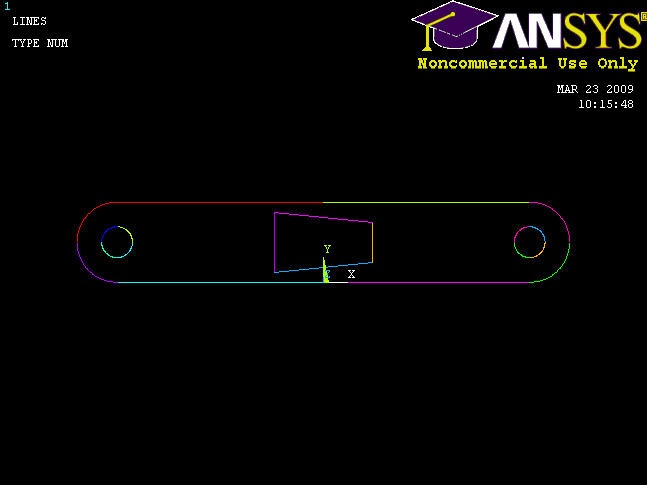
Next, we want to fillet the corners, as specified in the drawing.
You can zoom in and out by using the mouse wheel or clicking on the appropriate buttons on the right toolbar (magnifying glass with + or -).
Main Menu > Preprocessor > Modeling > Create > Lines > Line Fillet
Pick two lines that meet at a corner where you want to put a fillet, then click OK. Enter a Fillet radius of 0.177, and click Apply. Repeat for the other three corners of the quadrilateral. Compare results with image below.

Finishing the Crank Face
All that's left now is to create a new area from the filleted quadrilateral region, and then subtract it from the rest of the crank face.
Main Menu > Preprocessor > Modeling > Create > Areas > Arbitrary > By Lines
In the Pick window, select Loop. Click on any of the line segments that we have just created and the entire cutout region should be selected. Click OK. Switch back to area view by going to
Utility Menu > Plot > Areas
Subtract out the new area from the rest of the crank by the same procedure as before.
Main Menu > Preprocessor > Modeling > Operate > Booleans > Subtract > Areas
Select the rest of the crank face, then OK.
It will be helpful to hold down the left mouse-button while picking an area, as an area changes color when it is selected. Move the pointer until the desired area is highlighted, then release the button. Finally, select the new cut-out area, then press OK again.
The result:

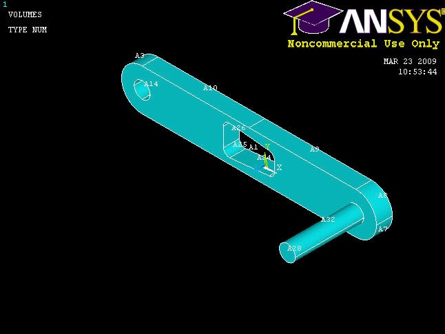
Creating the Volume
We will now make the face 3-D by extruding it by a given offset distance, similar to modeling in CAD.
Main Menu > Preprocessor > Modeling > Operate > Extrude > Areas > By XYZ Offset
Click Pick All. In the following window, change the DZ offset to 0.5. Click OK. To see your finished work, go to
Utility Menu > Plot > Volumes
Then click on the isometric view button  on the right toolbar.


Creating the Pedal Shaft
Main Menu > Preprocessor > Modeling > Create > Volumes > Cylinder > Solid Cylinder
Enter the following values and press OK.

We must now glue the shaft to the crank. The reason for using "glue" instead of performing a boolean add on the volumes is to maintain two discrete parts. This provides more flexibility in modeling, as it can allow for different materials and meshes. Note: If glue is not used, the two pieces will be independent of each other and the solution will be incorrect.
Main Menu > Preprocessor > Modeling > Operate > Booleans > Glue > Volumes
Click Pick All to glue our two volumes together. Note that there are no visual indicators of whether or not the volumes have been glued. You should check the Command Window and look for the "GLUE VOLUMES" command.

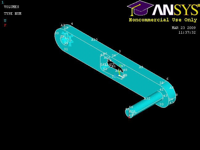
Your complete crank model should now look like this:

Save Your Work
Toolbar > SAVE_DB
See and rate the complete Learning Module
Go to all ANSYS Learning Modules
Step 5: Mesh geometry
Bring up the MeshTool:
Main Menu > Preprocessor > Meshing > MeshTool
We'll first mesh the two front surfaces using MESH200. Click Set next to Global under Element Attributes. Set the TYPE to MESH200 and click OK.

According to the ANSYS manual, "Smart element sizing (SmartSizing) is a meshing feature that creates initial element sizes for free meshing operations. SmartSizing gives the mesher a better chance of creating reasonably shaped elements during automatic mesh generation ... The SmartSizing algorithm first computes estimated element edge lengths for all lines in the areas or volumes being meshed. The edge lengths on these lines are then refined for curvature and proximity of features in the geometry." To turn on SmartSizing, check the box next to Smart Size. Drag the slider to a size of 4 to get a finer mesh than the default.
In order to have a little more control over what mesh ANSYS creates for us, we will set the starting element size for SmartSizing rather than use the default. Smartsizing will take this starting element size and modify/vary it over the geometry to account for curvature and corners. Under Size Controls, click the Set button next to Global. Enter an element edge length of 0.12 and click OK. The specified smart size of 4 and edge length of 0.12 are the result of an iterative process. You should experiment with different settings for these parameters to study the effect of the mesh on your solution, as discussed in Step 9. The goal is to obtain a solution that doesn't change as you refine the mesh.

Select Areas to be meshed with a Quad shape using the Free mesher. Click Mesh. Pick the front face of the crank and the pedal shaft.

Click OK. You will now see:

You'll get the following warning:

Elements that exceed shape warning limits can lead to degraded accuracy. Here it is a minor concern since only 1 element out of 682 is causing the warning. So it is reasonable to press on. In general, it is always a good idea to pay close attention to the warnings and understand their effect on your solution. As a veteran in these things, I can attest that ignoring warnings can come back to bite you in incovenient parts of the anatomy. Close the warning window.
In the above, we chose the front faces of the crank arm and pedal shaft as the surface meshes for sweeping. However, we have found that for other crank geometries, when meshing using the MESH200 elements, it is a good idea to choose the two back faces of the crank arm and pedal shaft that are flush with each other (i.e. the negative-z faces). This ensures that the nodes around the circumference of the circle on the two parts will match up and may prevent problems in sweeping the volume elements.
Bring up the MeshTool again. Click Set next to Global under Element Attributes. Set the TYPE to SOLID45 and click OK. We want four layers of mesh elements to span the thickness of the crank, so the desired element edge length in the sweep direction is (0.5 /4) = 0.125 in. Under Size Controls, click the Set button next to Global. Enter an element edge length of 0.125 and click OK. We will now sweep, i.e. extrude, the surface meshes created above across the corresponding volumes. Select Volumes to be meshed with a Hex shape along with the Sweep option as shown below. Make sure Auto Src/Trg is selected; this will automatically pick a source (Src) surface mesh and sweep/extrude it to a target (Trg) surface.

Click Sweep and Pick All to sweep-mesh both volumes. ANSYS will extend our previous surface meshes across the corresponding volumes.

ANSYS issues a warning that 5 out of 3986 elements violate shape warning limits. Since the number of "bad" elements is small, this is a minor concern and we'll press on. But keep in mind that what we'll obtain is a reasonable first-cut solution but it will not be the final word. For that, you'll have to show that the solution is independent of the mesh. Close the warning window and the Meshtool.
Save Your Work
Toolbar > SAVE_DB
Go to Step 6: Specify boundary conditions
See and rate the complete Learning Module
Go to all ANSYS Learning Modules
Step 6: Specify boundary conditions
We have two loading conditions to specify. First we must fix the hole where the crank would attach to the bicycle. Then we apply our loading condition of 100 lb on the end of the shaft.
Fixed End
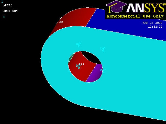
Main Menu > Preprocessor > Loads > Define Loads > Apply > Structural > Displacement > On Areas
It will be helpful to see the areas we're constraining, so select Utility Menu > Plot > Areas. We can see that the hole consists of multiple areas (4, in fact). Hold down the left-click and you can see that there are 4 surfaces that make up the inside of the hole. Pick all 4 and click OK. Select All DOF and click OK. The displacement value can be left blank as it defaults to 0. Symbols appear at the centers of each constrained area indicating that the area is constrained in three directions.

Force on Shaft
Main Menu > Preprocessor > Loads > Define Loads > Apply > Structural > Force/Moment > On Keypoints
Select Utility Menu > PlotCtrls > Numbering ... and turn On Keypoint Numbers. Click OK. Notice that there is conveniently a keypoint at the tip of the shaft, and pick this point to apply the force. Click OK. From the orientation of our axes, we want a constant force in the FY direction with a value of -100. Click OK.
What the model looks like now:

Now let's see some results!
Save Your Work
Toolbar > SAVE_DB
See and rate the complete Learning Module
Go to all ANSYS Learning Modules
Step 7: Solve!
Before we start the solution, we should check our model for errors. Enter check in the Input window and press Enter.

All warnings and errors found will be displayed in the Output Window. There are no errors but you will see the warnings regarding element shapes that we encountered before. So we're finally ready to kick back and let ANSYS do some of the work: assembling the local and global stiffness matrices and inverting the global system to determine the displacements at the nodes.
Main Menu > Solution > Solve > Current LS
Click OK in Solve Current Load Step menu.

ANSYS should cheerfully report "Solution is done!"
Verify that ANSYS has created a file called crank.rst in your working directory. This file contains the results of the (previous) solve.
Go to Step 8: Postprocess the results
See and rate the complete Learning Module
Go to all ANSYS Learning Modules
Step 8: Postprocess the Results
Plot Deformed Shape
Main Menu > General Postproc > Plot Results > Deformed Shape
Select Def + undef edge and click OK.
This plots the deformed and undeformed shapes in the Graphics window. The maximum deformation DMX is 0.026148 inches as reported in the Graphics window. We should check that our results make sense. It appears that the boundary conditions have been satisfied as the tip of the shaft moves downward and the hole at the other end of the crank is held in place.

Animate the deformation
Utility Menu > PlotCtrls > Animate > Deformed Shape...
Select Def + undeformed and click OK. Select Forward Only in the Animation Controller. This is also a good way to check the boundary conditions have been applied correctly. Close the Animation Controller.
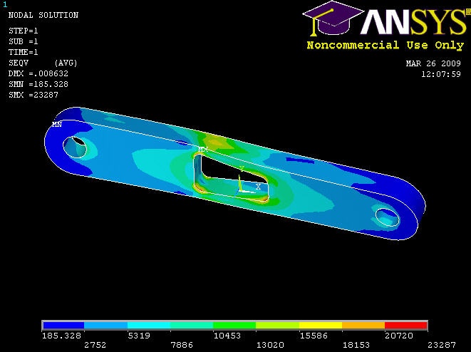
Plot Nodal Solution of von Mises Stress
For a quick refresher on von Mises stress, click Help. Search for von mises and click on the result 2.4 Combined Stresses and Strains (this is lower down among the search results). Read through section 2.4.2.
Main Menu > General Postproc > Plot results > Contour Plot > Nodal Solu
Select Nodal Solution > Stress > von Mises stress and click OK. To change the range of stresses displayed, go to
Utility Menu > PlotCtrls > Style > Contours > Uniform Contours ...
and select User specified. Specify a range of minimum 0 and maximum 25000. We can now see more color variation in the model, and easily pick out the red areas.
When you plot the "Nodal Solution", ANSYS obtains a continuous distribution as follows:
1. It determines the average at each node of the values of all elements connected to the node.
2. Within each element, it linearly interpolates the average nodal values obtained in the previous step.
This procedure is in effect a smoothing operation.
The stress concentration located at the tip of the shaft can be ignored as the force is applied as a point load. Let's look at the results just for the crank by deselecting the elements within the pedal shaft volume. Go to
Utility menu > Select > Entities ...
Select Volumes, By Num/Pick, From Full and click Apply. Pick the crank volume and click OK. After we've selected a volume, we must next select all the elements in this volume. In the Select Entities window, select Elements, Attached to, Volumes and click Apply. Click Replot to display the new selection. Notice the deformation is exaggerated, revealing that deformation is primarily caused by torsion.

To select the whole model again, go to Utility Menu > Select > Everything.
Comparing the σxx Stress with von Mises Stress
To verify that the bending stress in the crank is relatively insignificant, we can compare the element σxx solution with the elemental von Mises solution.
General Postproc > Plot Results > Contour Plot > Element Solu
Click on Stress, then X-Component of stress , then Apply.
If grey areas are appearing in your contour plots, you should go to Utility Menu > PlotCtrls > Style > Contours > Uniform Contours ..., select Auto calculated, and click OK.
Notice that the top-left and bottom-right corners of the cutout area are now blue, and that the scale has been readjusted to show that blue is now a large negative stress value. If this were a case of pure bending, we would expect the top of the crank to be in tension, not compression!
To find out information about specific points on the model, go to
General Postproc > Query Results > Subgrid Solu
Select Stress, X-direction SX, and click OK. The picking window will appear, and you can click on any point in the model. Click OK when finished.

Compare the stress values with the von Mises stress. (Click on von Mises stress, then OK)
Investigate the Stress Concentration
Let's zoom in on the red area. Use the mouse wheel to zoom in and out in the view area. Some other viewing functions: Holding down the Ctrl key and the left mouse button allows you to pan the view, while holding the Ctrl key and the right mouse button allows you to rotate the view. Hold down the right mouse button and draw a rectangle to zoom in on a specific region.
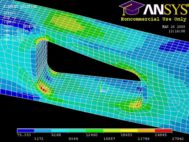
Recall that the nodal solution shows smoothed stress values. Let's compare the nodal solution with the element, i.e. non-smoothed, solution.
General Postproc > Plot Results > Contour Plot > Element Solu
Click on Stress, then von Mises Stress, then the OK button. In the vicinity of the cut-out corners, there are fairly significant discontinuities in the von Mises stress across adjacent elements. This suggests that we need to refine the mesh at least in this region. This is done in the next step.

Calculate Average Strain in Specified Area
In a perfect world, we would be able to validate the ANSYS results by comparing them with strain gage measurements at selected locations. We unfortunately don't have strain gage measurements for this particular geometry but will anyway show you the process by which you can calculate the average strain over an area where a strain gage would be placed. This will help prepare you to compare your ANSYS results with strain gage measurements for a different geometry for which you may have experimental data.
Let's assume that the strain gage is placed on the front face of the crank (z=0.5") roughly halfway between the left hole and the cutout as shown below.

In the coordinate system in our model, let's say this area is given by -1.77"≤ x≤ -1.57" and 0.45"≤ y≤ 0.85". To find the average strain in this area, we will select all nodes that lie in this area and then list the strain values at these nodes. You can copy these values over to Excel or MATLAB to find the average value.
ANSYS provides extensive capabilities, referred to as "select logic", for selecting a subset of the full model using various criteria. We'll use select logic to select the nodes on the front face of the crank. We'll first select the area corresponding to this face.
Utility Menu > Plot > Areas
Utility Menu > Select > Entities
Select Areas from the pull-down menu at the top. Make sure By Num/Pick is selected below that. Click Apply.

Hold down the left mouse button until the front face is picked. Click OK in the pick menu.

Only the area corresponding to this face is selected currently. Verify this by clicking Replot in the Select Entities menu (this replots areas).
One key thing to remember about ANSYS' "select logic" is that the various entity types (areas, volumes, nodes, elements, etc) are selected independently. So all nodes are still "selected", not just the ones that are located on the front face of the crank. Verify this: Utility Menu > Plot > Nodes.
We next select the nodes attached to the previously selected area. In the Select Entities menu, select Nodes from the pull-down menu at the top and Attached to below that. Select Areas, All below that. Click Apply.

Check that only nodes attached to the front face are currently selected by clicking Replot in the Select Entities menu (this replots nodes).
We can get a better idea of where these nodes are located by plotting nodes as well as lines.
Utility Menu > PlotCtrls > Multi-Plot Controls ... > OK
Select Lines and Nodes and click OK.
Utility Menu > Plot > Multi-Plots

From these currently selected nodes, we next select nodes that satisfy the following criterion: -1.77"≤ x≤ -1.57". In the Select Entities menu, retain Nodes at the top. Select By Location and X coordinates below that. Enter Min,Max values as per the snapshot below. Since we want the nodes to be selected from the current set rather than the full set, choose the Reselect radio button. Click Apply and then Replot.

You should see that only the nodes that are in the desired x-coordinate range are selected.

Save your work:Toolbar > SAVE_DB
Next, from the current set of nodes, select nodes that satisfy the following criterion: 0.45"≤ y≤ 0.85" by appropriately modifying the previous select action step. The snapshot below shows what I get: four nodes remain in the selected set. If you mess up, resume from your .db file.

Now all actions on nodes will be performed only on the four nodes that are currently selected. For instance, to list the strain values at these nodes, choose
Main Menu > General Postproc > List results > Nodal Solution > Elastic Strain > X-Component of elastic strain
You can save these values to a text file using File > Save as. You can then read in the values from the text file into Excel or MATLAB for further processing such as finding the average.
Once you are done with the select operations, exit the Select Entities menu and choose
Utility Menu > Select > Everything
Utility Menu > Plot > Nodes
Save your work:Toolbar > SAVE_DB
Go to Step 9: Validate the results
See and rate the complete Learning Module
Go to all ANSYS Learning Modules
Step 9: Validate the results
It is very important that you take the time to check the validity of your solution. This section leads you through some of the steps you can take to validate your solution.
Simple Checks
Does the deformed shape look reasonable and agree with the applied boundary conditions? We checked this in step 8.
Do the reactions at the supports balance the applied forces for static equilibrium? To check this, select
Main Menu > General Postproc > List Results > Reaction Solu
Select All struc forc F for Item to be listed and click OK. The forces in the X and Z directions are essentially zero and the total Y-reaction is 100.00 (lbf) as expected.
Refine Mesh
Let's repeat the solution on a finer mesh with more divisions in the z-direction. Repeat the mesh steps for the MESH200 element, but this time use smart size 3 and element size of 0.08. Repeat the mesh steps for the SOLID45 element and set the element edge length to 0.05 instead of 0.125. This will create 10 divisions through the thickness of the crank instead of 4. When warned that the picked volumes are already meshed, check Yes and click OK to remesh.
Obtain a new solution and plot the elemental solution of the von Mises stress:

. |
Coarser Mesh |
Finer Mesh |
DMX |
0.026148in |
0.026651in |
SMX |
25308psi |
27942psi |
The maximum displacement at the tip of shaft is 1.9% greater and the maximum stress is 10% greater. This indicates that the solution we have obtained is still dependent on the mesh. We would need to further refine the mesh. Do keep in mind that one would have to make more detailed comparisons between the solutions on the two meshes before we can make a definitive statement about the mesh independence of our results.
Exit ANSYS
Utility Menu > File > Exit
Select Save Everything and click OK.