 Sign-up for free online course on ANSYS simulations!
Author: Rajesh Bhaskaran & Yong Sheng Khoo, Cornell University
Problem Specification
1. Pre-Analysis & Start-Up
2. Geometry
3. Mesh
4. Setup (Physics)
5. Solution
6. Results
7. Verification & Validation
This tutorial is no longer updated. Use the new bike crank tutorial instead.
Problem Specification
A preeminent bicycle company is disappointed with the negative feedback they have received on their latest model, and they have pinpointed the problem to an outdated bicycle crank design that they assumed would still withstand typical loads. To protect their reputation, they have outsourced the task of analyzing the crank to you, providing you with the geometry of the bicycle crank and attached pedal shaft shown below. The dimensions are given in inches. The material they selected has an Young's modulus E = 2.8x10⁷ psi and Poisson ratio ν=0.3.

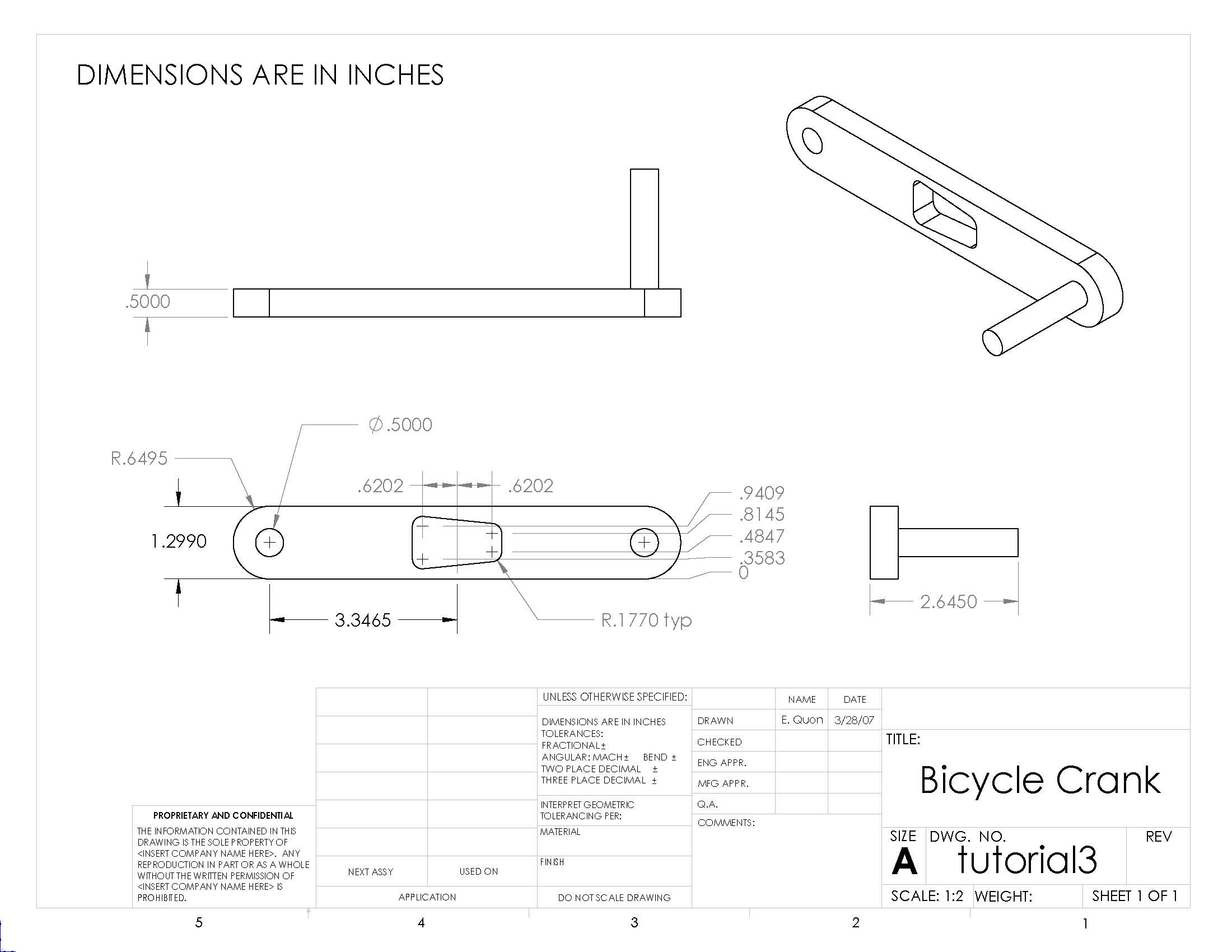
Using ANSYS, determine the mechanical response due to a load of 100 lbf applied vertically downward at the end of the pedal shaft as shown in the figure below. Assume that the crank is attached rigidly to a fixed shaft fitted into the hole near the left end of the crank. This means you can constrain the surface of the left hole in X, Y and Z directions as indicated below.

Calculate the deflection, strain and stress distributions in the crank/pedal shaft combination for this loading condition. Use the ANSYS results to evaluate the degree of stress concentration in the vicinity of the cut-out in the crank geometry.
Go to Step 1: Pre-Analysis & Start-Up
Author: Rajesh Bhaskaran & Yong Sheng Khoo, Cornell University
Problem Specification
1. Pre-Analysis & Start-Up
2. Geometry
3. Mesh
4. Setup (Physics)
5. Solution
6. Results
7. Verification & Validation
Step 1: Pre-Analysis & Start-Up
From the problem statement, we know that we are solving static structural problem.
Start ANSYS Workbench
With the new release of ANSYS 12, there have been a lot of improvement in term of overall flow. We start our simulation by first starting the ANSYS workbench.
Start > All Programs > ANSYS 12.0 > Workbench
Following figure shows the workbench window.

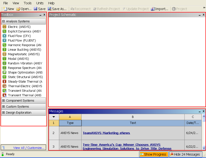
At the left hand side of the workbench window, you will see a toolbox full of various analysis systems. In the middle, you see an empty work space. This is the place where you will organize your project. At the bottom of the window, you see messages from ANSYS.
Select Analysis Systems


Since our problem involves static analysis, we will select the Static Structural (ANSYS) component on the left panel.
Left click (and hold) on Static Structural (ANSYS), and drag the icon to the empty space in the Project Schematic.
Since we selected Static Structural (ANSYS), each cell of the system corresponds to a step in the process of performing the ANSYS Structural analysis. Rename the project to Crank.

Now, we just need to work out each step from top down to get to the results for our solution.
- We start by preparing our geometry
- We use geometry to generate a mesh
- We setup the physics of the problem
- We run the problem in the solver to generate a solution
- Finally, we post process the solution to gain insight into the results
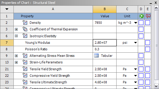
Specify Material Properties
We will first specify the material properties of the crank. The material has an Young's modulus E=2.8x10⁷ psi and Poisson's ratio ν=0.3.
In the Crank cell, double click on Engineering Data. This will bring you to a new page. The default material given is Structural Steel. We will use this material and change the Young's modulus and Poisson's ratio.
Left click on Structural Steel once and you will see the details of Structural Steel material properties under Properties of Outline Row 3: Structural Steel. Under Isotropic Elasticity, change Young's Modulus and Poisson's Ratio to E=2.8e7 psi and ν=0.3. Remember to change the unit accordingly.

Press the Return to Project  to return to Workbench Project Schematic window.
Author: Rajesh Bhaskaran & Yong Sheng Khoo, Cornell University
Problem Specification
1. Pre-Analysis & Start-Up
2. Geometry
3. Mesh
4. Setup (Physics)
5. Solution
6. Results
7. Verification & Validation
Step 2: Geometry
Note: You can import geometry from Solidworks. Just make sure that when you create your geometry in Solidworks, you have the Crank body and Handle body.
In the Crank cell, right click on Geometry, and click New Geometry...

At this point, a new window, ANSYS Design Modeler will be opened. You will be asked to select desired length unit. Select Inch unit and click OK.
Creating a Sketch
Like any other common CAD modeling practice, we start by creating a sketch.
Start by creating a sketch on the XYPlane. Under Tree Outline, select XYPlane, then click on Sketching next to Modeling tab. This will bring up the Sketching Toolboxes.
Note: In sketching mode, there is Undo features that you can use if you make any mistake.

On the right, there is a Graphic window. At the lower right hand corner of the Graphic window, click on the +Z axis to have a normal look of the XY Plane.

Under Sketching Toolboxes, click on Draw tab. We will first create the outline of the crank. Select Rectangle and draw in the Graphics window as shown below. Make sure that the rectangle is coincident with the x-axis (Letter C will appear).

Note: You do not have to worry about dimensions for now, we can dimension them properly in the later step. Next draw the semi-circular arc at both end of rectangle. Under Draw Tab, select Arc by Center and execute the drawing as shown.

Draw the crank circular hole next. Under Draw tab, click on Circle and execute the drawing as shown.

Next, we will dimension the current drawing. Under Sketching Toolboxes, select Dimensions tab. You will see a list of dimensioning options. We will use the default General option. Execute the geometry dimensioning as shown below.

Input value for D2, H3, L1 respectively under Details View tab.
D2 = 0.5 in
H3 = 3.3465 in
L1 = 1.299 in
Note: Your dimension naming might not be the same as the one shown here. It is fine. Just make sure your value correspond to correct dimensions.
Next, we need to make sure that the sketch is symmetric on both side. Under Sketching Toolboxes, select Constraints tab. Select Midpoint and constrain the geometry in the Graphics window as shown below.

Next, we will make sure that the both circular hole is of same dimension. Under Constraints tab, select Equal Radius. Execute constraint in the Graphics window as shown below.

We will next trim off the unwanted edge. Under Modify tab, select Trim. Execute the trimming in Graphics window as shown below.

At this point, we have the outline of the crank done. We need to add the cut out in the middle of the crank. First start with a sketching of the cut-out. Under Draw tab, click on Line and execute drawing in Graphic window as shown below.

We would want the four corners of the cut out we created to be of following coordinate.
(-0.7972, 0.1642)
(0.7972, 0.3248)
(0.7972, 0.9744)
(-0.7972, 1.1368)
Unfortunately, there is no easy way in specifying the coordinates of a point. So we will have to dimension them accordingly using the dimensioning tools. Click on Dimensions tab and use General tool and execute the dimensioning as shown.

Under Details View, enter the value for the dimensions.
H5 = 0.7972 in
H6 = 0.7972 in
L4 = 0.1642 in
L7 = 0.3248 in
L8 = 0.3248 in
L9 = 0.1642 in
Next we will add fillet to the corner of the cut out. Click on Modify tab and select Fillet. Enter a Radius value of 0.177 in. Execute the command in Graphics window as shown.

Now we have the sketch of the crank done. Next we will perform extrude feature on this sketch.
Create > Extrude
Under Details View, Sketched1 is automatically selected as default Base Object.
Next to FD1, Depth (>0), enter value 0.5 in. Click Generate.

Note that after you click Generate, you see a new part created under the Tree Outline. This is what you should have in the Graphics window at this point.

Now let's keep moving by adding a handle to this crank. Under Tree Outline, click on XY Plane and click on New Sketch  . This will create a new sketch under XY Plane. You will see Sketch2 created under XYPlane. Click on the Sketching tab to start sketching the handle. The base sketch for the handle is just a cycle. Under Draw tab, click on Circle.

Execute the drawing in the Graphics window as shown below.

At this point, we have the crank handle sketch done. We can continue adding Extrude feature to the sketch. Click Extrude, make sure that Sketch2 is selected next to Base Object. Next to Operation change Add Material to Add Frozen. This is because we want to create the crank as two separate bodies. If we use the default Add Material, both the crank and crank handle will be created as a single body. Next to FD1, Depth (>0) enter value of 2.645. We can now Generate this feature. Under Tree Outline, you will see that we now have 2 Parts and 2 Bodies. Select both parts and perform Form New Part operation.

In the Graphics window, this is what you should have now.

Congratulations! We are done with the Geometry setup. Let's close the Design Modeler and go back to the Workbench (Your work will be saved. Don't worry).
Author: Rajesh Bhaskaran & Yong Sheng Khoo, Cornell University
Problem Specification
1. Pre-Analysis & Start-Up
2. Geometry
3. Mesh
4. Setup (Physics)
5. Solution
6. Results
7. Verification & Validation
Step 3: Mesh
In the Crank cell, right click on Model, and click Edit...
A new window Mechanical Modeler will open. We will start with the default mesh generation method. Under Outline, right click on Mesh and click Generate Mesh. This will give us mesh that ANSYS mesher thinks appropriate for our geometry. We see that ANSYS is smart enough to create a mesh that sweep across the cross sectional area of the crank. This is the type of mesh we are seeking for our geometry. However, sizing wise, the mesh is too coarse. We will have to increase the number of elements.
Under Outline, click on Mesh. Next under Details of "Mesh", expand the Sizing tab and we will specify the element size that we desire. Element size of 0.125 in seems to be a good start. Next to Element Size, enter 0.125. Finally, click on Generate Mesh again.

This is the mesh that appear in the Graphics window on the right.

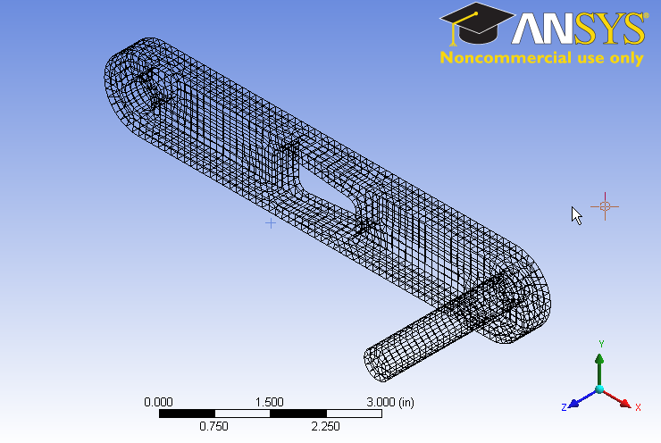
You should have 18205 nodes and 3582 elements for your mesh. Click on Statistics under Details of "Mesh" to see that.
For future reference, the default mesh might not produce the desirable mesh that we want. To specify our own mesh control, right click on Mesh and select Insert. This way, we can insert meshing type and control that we desire. To learn more about different meshing methods, please refer to the Mechanical Help at the top menu.
Author: Rajesh Bhaskaran & Yong Sheng Khoo, Cornell University
Problem Specification
1. Pre-Analysis & Start-Up
2. Geometry
3. Mesh
4. Setup (Physics)
5. Solution
6. Results
7. Verification & Validation
Step 4: Setup (Physics)
We have two loading conditions to specify. First we must fix the hole where the crank would attach to the bicycle. Then we apply our loading condition of 100 lb on the end of the shaft.
Fixed Support
Under Outline, right click on Static Structural (F5), move the mouse cursor to Insert and select Fixed Support.
Now in the Graphics area, select the cylindrical hole and click Apply next to the Geometry under Details of "Fixed Support". You will see the fixed support boundary condition shown in the Graphics window.

Force on Shaft
Now we will apply 100 lb force at the end of the shaft. This time, I will show you another way of inserting boundary condition.
Under Outline, left click on Static Structural (F5). Third menu at the top will show different type of boundary conditions. Left click on Loads and select Force. In the GraphicsDetails of "Force" window, select the circular area at the end of the shaft. Under , click Apply next to Geometry. The selected area in the Graphics window will be applied with this boundary condition. Next we will enter the value of 100 lb force. Next to Define By, change Vector to Components. Enter a value of -100 next to Y Component. In the Graphics window, you will see the direction of force applied.

Congratulations! We are done setting up the boundary conditions.
Author: Rajesh Bhaskaran & Yong Sheng Khoo, Cornell University
Problem Specification
1. Pre-Analysis & Start-Up
2. Geometry
3. Mesh
4. Setup (Physics)
5. Solution
6. Results
7. Verification & Validation
Step 5: Solution
Now that we have set up the boundary conditions, we can actually solve for a solution. Before we do that, let's take a minute to think about what is the post-processing that we are interested in. We are interested in the deflection and stress on the crank. Let's set up those post-processing parameters before we click solve button.
Under Outline, left click on Solution (F6). At the top third menu, insert Total Deformation and von Mises Stress. Finally click Solve at the top menu.

Author: Rajesh Bhaskaran & Yong Sheng Khoo, Cornell University
Problem Specification
1. Pre-Analysis & Start-Up
2. Geometry
3. Mesh
4. Setup (Physics)
5. Solution
6. Results
7. Verification & Validation
Step 6: Results
Total Deformation
Let first look at Total Deformation. Under Solution (F6), click on Total Deformation. The Total Deformation plot is then shown in the Graphics window. The maximum deflection is 0.026644 in. We should check that our results make sense. It appears that the boundary conditions have been satisfied as the tip of the shaft moves downward and the hole at the other end of the crank is held in place.

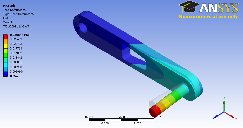
Note: To show the original undeformed crank, go to third menu click  and click on
Notice the deformation is exaggerated, revealing that deformation is primarily caused by torsion.
You can also animate the deformation by clicking play button right under Graphics window.

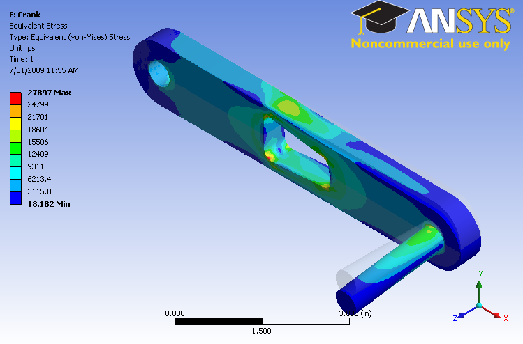
Von Mises Stress
Now let's look at the stress on the crank. Left clicking on Equivalent Stress under Solution (F6). In the Graphics window show the crank stress contour. The maximum stress is 27897 psi.

Here's the view without the handle.

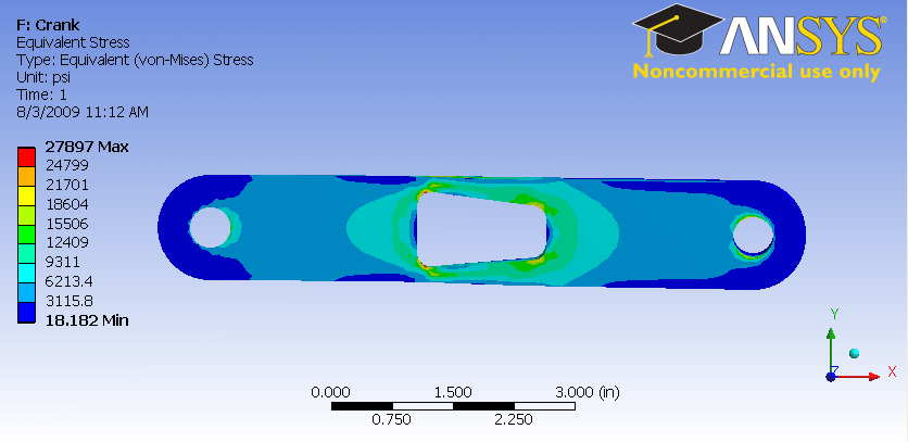
Note: To hide the crank handle, select the appropriate body in the Graphics window and right click and select Hide Body. Do the same to unhide a body.
Go to Step 7: Verification & Validation
Author: Rajesh Bhaskaran & Yong Sheng Khoo, Cornell University
Problem Specification
1. Pre-Analysis & Start-Up
2. Geometry
3. Mesh
4. Setup (Physics)
5. Solution
6. Results
7. Verification & Validation
Step 7: Verification & Validation
It is very important that you take the time to check the validity of your solution. This section leads you through some of the steps you can take to validate your solution.
Simple Checks
Does the deformed shape look reasonable and agree with the applied boundary conditions? We checked this in step 6.
Do the reactions at the supports balance the applied forces for static equilibrium? To check this, select
Outline > Solution (F6) > Insert > Probe > Force Reaction
Under Details of "Force Reaction", select Fixed Support as Boundary Condition. At the top menu, click Solve to Evaluate All Results.
The forces in the X and Z directions are essentially zero and the total Y Axis is 100.00 (lbf) as expected.
Refine Mesh
Let's repeat the solution on a finer mesh with more smaller element size. Repeat the mesh steps, but this time use element size of 0.05 instead of 0.125. This will create 10 divisions through the thickness of the crank instead of 4.
Obtain a new solution and compare both solution.
. |
Coarser Mesh |
Finer Mesh |
Max Deformation |
0.0257in |
0.0258in |
Max Stress |
27897psi |
27978psi |
The difference in maximum displacement at the tip of the crank handle is less than 0.4%.
The difference in maximum stress at the cut out area is less than 0.3%.
This means that our mesh is refine enough and the solution obtained using the original mesh is probably good enough.
Do keep in mind that one would have to make more detailed comparisons between the solutions on the two meshes before we can make a definitive statement about the mesh independence of our results.