ANSYS 12 - 2D Steady Conduction - Results

6. Results

If necessary , download the solution by right-clicking the following link: conduction 2d.zip

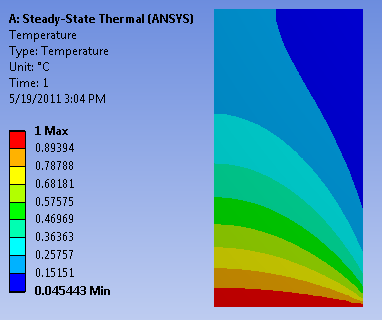
Temperature

To view the temperature distribution over the surface, select Solution > Temperature from the tree on the left.

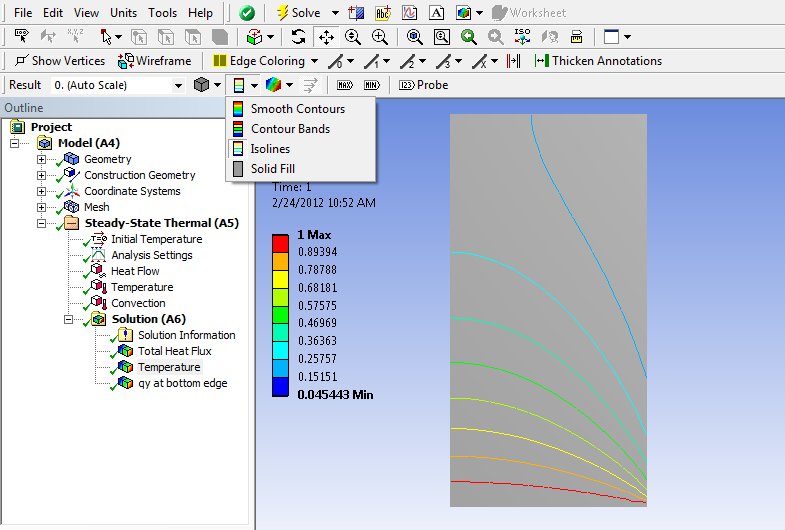
In order to view the contours as isolines, select the viewing button, and change from Contour Bands into Isolines.

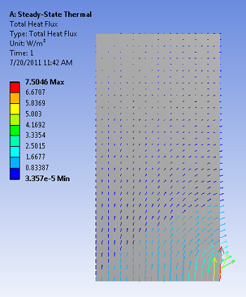
Total Heat Flux

We will view the heat flux as vectors. This will tell us the direction of heat flow within the geometry as well as at the boundaries  In order to plot the heat flux vectors, select Solution > Total Heat Flux from the tree on the left. Then (Click) Vectors, near the top of the GUI. The sliders in the top bar can be used to change the size and number of vectors displayed. At this point, the heat flux vectors should appear similar to the image below. Take a minute to think about whether the heat flow directions at the boundaries match what you expect.

Temperature along Y=1m line

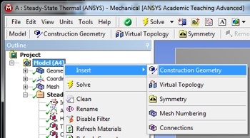
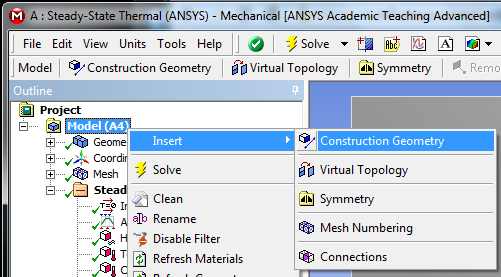
Let us extract the temperature values along the horizontal line, y=1m. This is done by defining a "path" corresponding to y=1m and sampling the temperature along this path. First, (Right Click) Model > Insert > Construction Geometry as shown below.

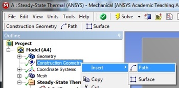
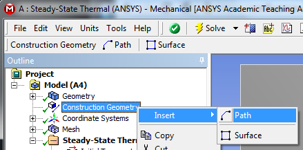
Next, (Right Click) Construction Geometry > Insert > Path as shown in the following image.




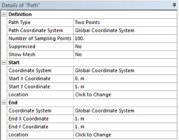
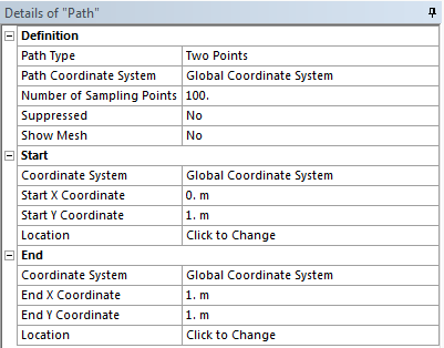
Then, set Number of Sampling Points to 100. Set Start X Coordinate to 0, set Start Y Coordinate to 1, set End X Coordinate to 1, and set End Y Coordinate to 1 as shown below. This sets the start and end points for the path.




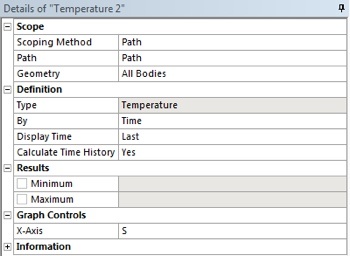
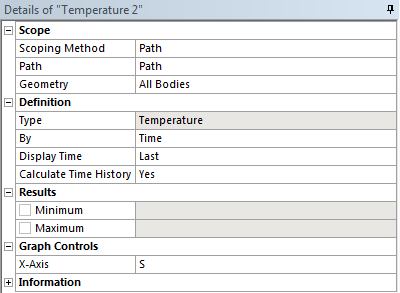
At this point another temperature output must be created under Solution in the tree. In order to create this temperature output, (Right Click) Solution > Insert > Thermal > Temperature. In the "Details of Temperature 2" table set the Scoping Method to Path as shown below. Then, set Path to Path (the default name for the path that was just created is path.) Your "Details of Temperature 2" table should now look like the following image.




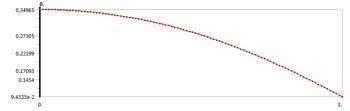
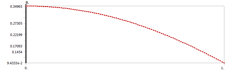
(Click) Solve, , and ANSYS will find the temperature on the line y=1 m as a function of the distance along the path, which in this case is the x position. ANSYS will obtain the temperature for 100 points on the line y=1m. The data points are displayed in a table and can be exported to a text file or EXCEL file by right-clicking on the table. The following image shows the graph that ANSYS outputs. The y axis is non-dimensional temperature and the x axis is x position on the line y=1m.

Directional Heat Flux along Y=0m line

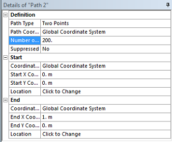
Now we are interested in calculating the heat flux through the bottom boundary.  First, construct a path, following steps similar to those above, but with the start and end points at the bottom corners of the surface. (Right Click) Model > Insert > Construction Geometry.  Next, (Right Click) Construction Geometry > Insert > Path. Then, set Number of Sampling Points to 200, set Start X Coordinate to 0, set Start Y Coordinate to 0, set End X Coordinate to 1, and set End Y Coordinate to 0 as shown below.

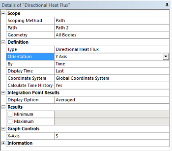
Similar to the Temperature inserted along the first path, now insert Directional Heat Flux results along Path 2. (Right Click) Solution > Insert > Thermal > Directional Heat Flux. Choose Path for the Scoping Method, set Path 2 for the Path and Y axis for Orientation, as seen below.

(Click) Solve,  , and ANSYS will find the Directional Heat Flux on the line y=0m as a function of x position.  We would like to find the total heat flux through the bottom by integrating the flux along that boundary. To do this we will export the data to MATLAB and perform a numerical integration.  Right click in the tabular data displayed in the lower righthand corner of the screen.  Select all (Ctrl+A), right-click and select Export.  Save the file as "qy_bot.txt" in your MATLAB working directory.

Next, open MATLAB and use the following code to integrate along the path:

clear all; clc;
qy_bot = dlmread('qy_bot.txt', '', 'B2..C50');
qy_bot_tot = trapz(qy_bot(:,1),qy_bot(:,2));

The dlmread function is used to read the data from the text file, while the trapz function performs numerical integration using trapezoids.  The variable 'qy_bot_tot' calculated in MATLAB represents the total dimensionless heat flux through the bottom, y=0 line.

Save

Save the project now.

 
Go to Step 7: Verification and Validation

See and rate the complete Learning Module

Go to all ANSYS Learning Modules