 Sign-up for free online course on ANSYS simulations!
Unable to render {include} The included page could not be found.
Author: John Singleton, Cornell University
Problem Specification
1. Pre-Analysis & Start-Up
2. Geometry
3. Mesh
4. Setup (Physics)
5. Solution
6. Results
7. Verification and Validation
Exercises
7. Verification and Validation
Verification and validation can be thought as a formal process for checking results. We'll first check that the net heat flow to the domain is zero. Then we'll look into mesh refinement and comparison with the analytical solution.
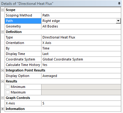
In order to check that the net heat flow to the domain is zero, we need to export the data from the bottom and right edges to MATLAB for numerical integration. Insert Directional Heat Flux results along the Right Edge. (Right Click) Solution > Insert > Thermal > Directional Heat Flux. Rename this result qx at right edge.
Choose Path for the Scoping Method, set Right Edge for the Path and X axis for Orientation, as seen below.

The next step is to export the data to text files that can be read into MATLAB. To do so, select qy at bottom edge. In the tabular data displayed in the bottom right corner, (Right Click)> Export. Save the file as qy_bot.txt on the Desktop. Similarly, save the data for qx at right edge as qx_right.txt.
We have written a MATLAB script that reads in the ANSYS results for heat flux along the bottom and right edges and does the necessary integration to calculate the total heat flow. Download the MATLAB script by right-clicking the link and saving to the Desktop: post.m. Running the file will graph the heat flux along each edge, as well as calculating the total heat flow through each of the two edges.
We will also look at the results for the dimensionless temperature along the line y=1. The plot below contains, the analytical solution, and the ANSYS solution for three different meshes.


As one can see, the ANSYS solution for the first mesh (10x20) is already mesh converged. In other words, refinements of the first mesh do not significantly change the solution. Furthermore, all three ANSYS solutions match the analytical solution quite well. It is very difficult to discern the different plots, letting us know that ANSYS is matching the analytical solution quite well.
Go to Exercises
See and rate the complete Learning Module
Go to all ANSYS Learning Modules