 Sign-up for free online course on ANSYS simulations!
FLUENT - Turbulent Pipe Flow - Step 5
Useful Information
Click here for the FLUENT 6.3.26 version.
Step 5: Solution
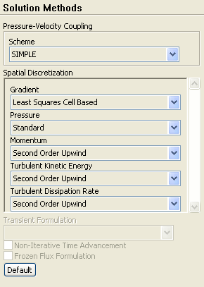
We'll use second-order discretization for the momentum equation, as in the laminar pipe flow tutorial, and also for the turbulence kinetic energy equation which is part of the k-epsilonturbulence model.
Problem Setup > Solution Methods
Change the Discretization for Momentum, Turbulence Kinetic Energy and Turbulence Dissipation Rateequations to Second Order Upwind (if you do not see all of the equations scroll down to see them).
|
Set Convergence Criteria
Recall that FLUENT reports a residual for each governing equation being solved. The residual is a measure of how well the current solution satisfies the discrete form of each governing equation. We'll iterate the solution until the residual for each equation falls below 1e-6.
Problem Setup > Solution > Monitors > Residuals, Statistic and Force Monitors
Double click on Residuals.Notice that Convergence Criterion has to be set for the k and epsilonequations in addition to the three equations in the last tutorial. Set the Convergence Criterionto be 1e-06 for all five equations being solved.
Select Print to Console and Plotunder Options. This will print as well plot the residuals as they are calculated which you will use to monitor convergence.
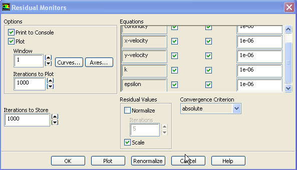
Click OK.
Set Initial Guess
We'll use an initial guess that is constant over the entire flow domain and equal to the values at the inlet:
Problem Setup > Solution > Solution Initialization
In the Solution Initializationmenu that comes up, choose inletunder Compute From. The Axial Velocityfor all cells will be set to 1 m/s, the Radial Velocity to 0 m/s and the Gauge Pressure to 0 Pa. The Turbulence Kinetic Energyand Dissipation Rate(scroll down to see it) values are set from the prescribed values for the Turbulence Intensity and Hydraulic Diameter at the inlet.
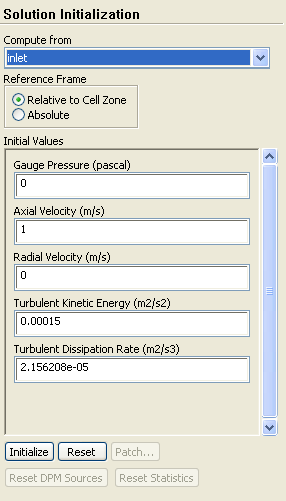
Click Initialize. Close the Solution Initializationwindow.
This completes the problem specification. Save your work:
Main Menu > File > Write > Case...
Type in {{pipe100x30.cas }}as the name of the Case File. Click OK. Check that the file has been created in your working directory.
Iterate Until Convergence
Solve for 100 iterations first.
Problem Setup > Solution > Run Calculation
In the Iterate menu that comes up, change the Number of Iterations to 100. Click Calculate.
You'll find that not all residuals have fallen below 1e-6 in 100 iterations. Solve for 200 more iterations. The solution converges in a total of about 210 iterations.
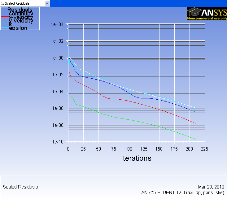
Click here to see a higher resolution image.
We need a larger number of iterations for convergence than in the laminar case since we have a finer mesh and are also solving additional equations from the turbulence model.
Save the solution to a data file:
Main Menu > File > Write > Data...
Enter pipe100x30.dat for Data File and click OK. Check that the file has been created in your working directory.
Go to Step 6: Results