FLUENT - Turbulent Pipe Flow - Step 4

Step 4: Setup (Physics)

If you have skipped the previous mesh generation steps 1-3, you can download the mesh by right-clicking on this link. Save the file as pipe100x30.msh. You can then proceed with the flow solution steps below.

Launch FLUENT

Lab Apps > FLUENT 6.3.26

Select 2ddp (2D, double-precision version) from the list of options and click Run.

Import File

Main Menu > File > Read > Case...

Navigate to your working directory and select the pipe100x30.msh file. Click OK.

The following should appear in the FLUENT window:

Check the number of nodes, faces (of different types) and cells. There are 3000 quadrilateral cells in this case. This is what we'd expect since we used 30 divisions in the radial direction and 100 divisions in the axial direction while generating the grid. So the total number of cells is 30*100 = 3000.

Also, take a look under zones. We can see the four zones inlet, outlet, wall, and that we defined in centerline GAMBIT.

Grid

First, we check the grid to make sure that there are no errors.

Main Menu > Grid > Check

Any errors in the grid would be reported at this time. Check the output and make sure that there are no errors reported. Then select:

Main Menu > Grid > Info > Size

The following summary about the grid should appear:

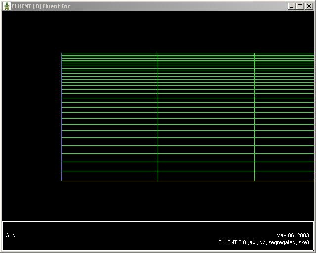
Let's look at the grid:

Main Menu > Display > Grid...

Make sure all 5 items under Surfaces are selected. Then click Display. Remember that we can zoom in using the middle mouse button. Zoom in and admire the grid. How many divisions are there in the radial direction?

Higher Resolution Image

Recall that you can look at specific components of the grid by choosing the entities you wish to view under Surfaces (click to select and click again to deselect a specific boundary). Click Display again when you have selected your boundaries. Use this feature and make sure that the boundary labels correspond to the correct geometric entities.

Close the Grid Display Window when you are done.

Define Governing Equations

Main Menu > Define > Models > Solver

Choose Axisymmetric under Space. As in the laminar pipe flow tutorial, we'll use the defaults of segregated solver, implicit formulation, steady flow and absolute velocity formulation. Click OK.

Main Menu > Define > Models > Energy...

The energy equation can be turned off since this is an incompressible flow and we are not interested in the temperature. Make sure no tick mark appears next to Energy Equation.

Main Menu > Define > Models > Viscous...

Choose k-epsilon (2eqn). Notice that the window expands and additional options are displayed on choosing the k-epsilon turbulence model. Under Near-Wall Treatment, pick Enhanced Wall Treatment so that we may get a more accurate result.

Click OK.
Main Menu > Define > Materials...

Change Density to 1.0 and Viscosity to *2e-5. These are the values in the Problem Specification. We'll take both as constant.

Click Change/Create.

Define Boundary Conditions

Main Menu > Define > Operating Conditions...

Recall that for all flows, FLUENT uses the gauge pressure internally. Any time an absolute pressure is needed, it is generated by adding the operating pressure to the gauge pressure. We'll use the default value of 1 atm (101,325 Pa) as the Operating Pressure.

Click Cancel to leave the default in place.

We'll now set the value of the velocity at the inlet and pressure at the outlet.

Main Menu > Define > Boundary Conditions...

The four types of boundaries we defined are specified as zones on the left side of the Boundary Conditions Window. Recall that we don't need to set any parameters for the centerline and wall zones. Verify this by selecting each of these two zones and clicking on Set....

Choose inlet and click on Set.... Enter 1 for Velocity Magnitude. This indicates that the fluid is coming in normal to the inlet at the rate of 1 meter per second. Select Intensity and Hydraulic Diameter next to the Turbulence Specification Method. Then enter 1 for Turbulence Intensity and 0.2 for Hydraulic Diameter. Click OK to set the velocity.

The (absolute) pressure at the outlet is 1 atm. Since the operating pressure is set to 1 atm, the outlet gauge pressure = outlet absolute pressure - operating pressure = 0. Choose outlet under Zone. The Type of this boundary is pressure-outlet. Click on Set.... The default value of the Gauge Pressure is 0. Click Cancel to leave the defaults in place.

Note: Backflow in the Pressure Outlet menu refers to flow entering through an outlet boundary. This is not likely to happen in this case. So we don't have to set the backflow parameters.

This completes the boundary condition specification. Close the Boundary Conditions menu.

Go to Step 5: Solution

See and rate the complete Learning Module

Go to all FLUENT Learning Modules