 Sign-up for free online course on ANSYS simulations!
Author: Rajesh Bhaskaran & Yong Sheng Khoo, Cornell University
Problem Specification
1. Pre-Analysis & Start-Up
2. Geometry
3. Mesh
4. Setup (Physics)
5. Solution
6. Results
7. Verification & Validation
Under Construction
The following ANSYS tutorial is under construction.
Problem Specification
Consider the beam in the figure below. There are two point forces acting on the beam in the negative y direction as shown. Note the dimensions of the beam. The Young's modulus of the material is 73 GPa and the Poisson ratio is 0.3. We'll assume that plane stress conditions apply.

Go to Step 1: Pre-Analysis & Start-Up
Author: Rajesh Bhaskaran & Yong Sheng Khoo, Cornell University
Problem Specification
1. Pre-Analysis & Start-Up
2. Geometry
3. Mesh
4. Setup (Physics)
5. Solution
6. Results
7. Verification & Validation
Step 1: Pre-Analysis & Start-Up
Start ANSYS Workbench
We start our simulation by first starting the ANSYS workbench.
Start > All Programs > ANSYS 12.1 > Workbench
Following figure shows the workbench window.

At the left hand side of the workbench window, you will see a toolbox full of various analysis systems. In the middle, you see an empty work space. This is the place where you will organize your project. At the bottom of the window, you see messages from ANSYS.
Select Analysis Systems

Since our problem involves static analysis, we will select the Static Structural (ANSYS) component on the left panel.
Left click (and hold) on Static Structural (ANSYS), and drag the icon to the empty space in the Project Schematic.
Since we selected Static Structural (ANSYS), each cell of the system corresponds to a step in the process of performing the ANSYS Structural analysis. Right click on Static Structural ANSYS and Rename the project to Beam.

Now, we just need to work out each step from top down to get to the results for our solution.
- We start by preparing our geometry
- We use geometry to generate a mesh
- We setup the physics of the problem
- We run the problem in the solver to generate a solution
- Finally, we post process the solution to gain insight into the results
Specify Material Properties
We will first specify the material properties of the crank. The material has an Young's modulus E=2.8x10⁷ psi and Poisson's ratio ν=0.3.
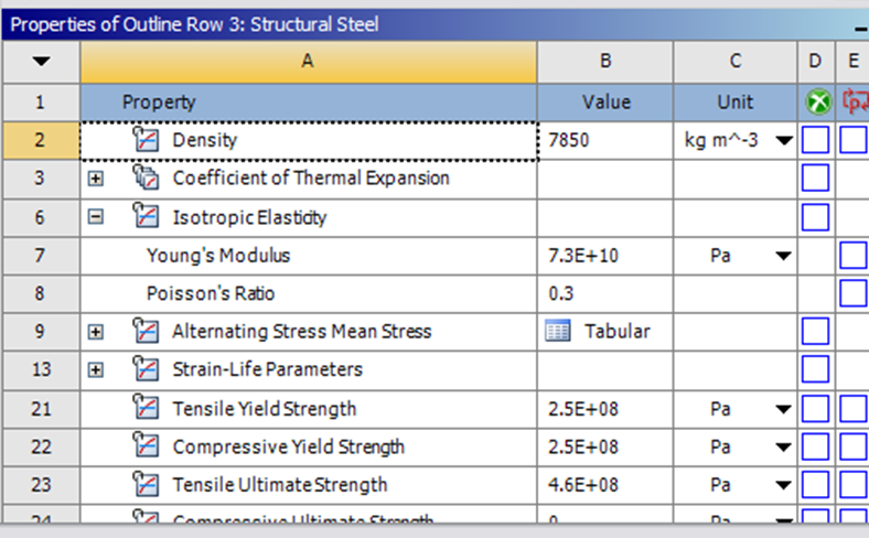
In the Crank cell, double click on Engineering Data. This will bring you to a new page. The default material given is Structural Steel. We will use this material and change the Young's modulus and Poisson's ratio.
Left click on Structural Steel once and you will see the details of Structural Steel material properties under Properties of Outline Row 3: Structural Steel. Expand Isotropic Elasticity, change Young's Modulus and Poisson's Ratio to E=7.9e10 pa and ν=0.3. Remember to check that you use the correct unit.

Press the Return to Project  to return to Workbench Project Schematic window.
Author: Rajesh Bhaskaran & Yong Sheng Khoo, Cornell University
Problem Specification
1. Pre-Analysis & Start-Up
2. Geometry
3. Mesh
4. Setup (Physics)
5. Solution
6. Results
7. Verification & Validation
Step 2: Geometry
Our geometry is 2D. At Workbench, in the Beam cell, right click on Geometry, and select Properties. You will see the properties menu on the right of the Workbench window. Under Advance Geometry Options, change the Analysis Type to 2D.

In the Project Schematic, double left click on Geometry to start preparing the geometry.
At this point, a new window, ANSYS Design Modeler will be opened. You will be asked to select desired length unit. Use the default meterunit and click OK.
Strategy for Geometry Creation
We need to apply point boundary conditions at four points A, B, C and D shown in the figure below. In ANSYS, point boundary conditions are applied to nodes. When we mesh the rectangle using the ANSYS Mesher, nodes will automatically be created at A and B since these are corner points; the corresponding displacement BC's can be applied to these corner nodes. However, there is no guarantee that there will be nodes exactly at C and D since these are not corners. In this case, ANSYS will apply the forces at the nodes that are closest to C and D. This is possibly acceptable if the mesh is sufficiently fine.

An alternative scenario is that we get clever and force C and D to be exact points. This can be done by splitting the top and bottom edges into three section as shown below. This will force nodes to be created at points C and D. Then, the point forces can be applied to these nodes. This is the strategy we'll use in creating the geometry.

Creating a Sketch
Like any other common CAD modeling practice, we start by creating a sketch.
Start by creating a sketch on the XYPlane. Under Tree Outline, select XYPlane, then click on Sketching next to Modeling tab. This will bring up the Sketching Toolboxes.
Note: In sketching mode, there is Undo features that you can use if you make any mistake.
On the right, there is a Graphic window. At the lower right hand corner of the Graphic window, click on the +Z axis to have a normal look of the XY Plane.
In the Sketching Toolboxes, select Rectangle. In the Graphicswindow, create a rough Rectangle from starting from the origin in the positive XY direction (Make sure that you see a letter P at the origin before you start dragging the rectangle. The letter P at the origin means the geometry is constrained at the origin.)
You should have something like this:

Note: You do not have to worry about geometry for now, we can dimension them properly in the later step.
Modify the Sketch
We would like to split the top and bottom with three edges. Click Modify tab and select Split. Roughly select four points on the top and bottom of the rectangle.

Dimensions and Constraints
Under Sketching Toolboxes, select Dimensions tab, use the default dimensioning tools. Dimension the geometry as shown:

Now we need to constraint the lower rectangle with the top of the rectangle which has been properly dimensioned. Click Constraints tab, select Equal Length. Click the appropriate top and bottom edge and set them to be of equal length.
Under Details View on the lower left corner, input the value for dimension appropriately.
V1: 0.05 m
H2: 0.1 m
H3: 0.2 m
H4: 0.1 m
At this point, you should see something like this for your sketch:

Create Surface
Now that we have the sketch done, we can create a surface for this sketch.
Concept > Surfaces From Sketches
This will create a new surface SurfaceSK1. Under Details View, select Sketch1 as Base Objects and click Apply. Finally click Generate ![]() to generate the surface. This is what you should see under your Tree Outline.
to generate the surface. This is what you should see under your Tree Outline.

You can close the Design Modeler and go back to Workbench (Don't worry, it will auto save).
Author: Rajesh Bhaskaran & Yong Sheng Khoo, Cornell University
Problem Specification
1. Pre-Analysis & Start-Up
2. Geometry
3. Mesh
4. Setup (Physics)
5. Solution
6. Results
7. Verification & Validation
Step 3: Mesh
Save your work in Workbench window. In the Workbench window, right click on Mesh, and click Edit. A new ANSYS Mesher window will open.
We would like to create a structured mesh where the opposite edges correspond with each other. Let's insert a Mapped Face mesh.
Outline > Mesh > Insert > Mapped Face Meshing
Under Outline, right click on Mesh, move cursor to Insert, and select Mapped Face Meshing. Finally select the beam surface body in the Graphics window and click Apply next to Geometry.
We can now generate the mesh using the default setting. Under Outline, right click on Mesh and click Generate Mesh. This should be the mesh appear in the Graphics window.


Under Details of "Mesh", you should see that we have 504 elements when you expand the Statistics tree.

Author: Rajesh Bhaskaran & Yong Sheng Khoo, Cornell University
Problem Specification
1. Pre-Analysis & Start-Up
2. Geometry
3. Mesh
4. Setup (Physics)
5. Solution
6. Results
7. Verification & Validation
Step 4: Setup (Physics)
We need to specify point BC's at A, B, C and D.

Let's start with setting up boundary condition at A.
Outline > Static Structural (A5) > Insert > Displacement
Select point A in the Graphics window and click Apply next to Geometry under Details of "Displacement". Enter 0 for both X Component and Y Component.

Let's move on to setting up boundary condition B.
Outline > Static Structural (A5) > Insert > Displacement
Select point B in the Graphics window and click Apply next to Geometry under Details of "Displacement 2". Enter 0 for Y Component and leave X Component to be free.

We can move on to setting up point force at point C and D.
Outline > Static Structural (A5) > Insert > Force
Select point C in the Graphics window and click Apply next to Geometry under Details of "Force". Next to Define By, change Vector to Components. Enter -4000 for Y Component.

Do the same for point D.
Author: Rajesh Bhaskaran & Yong Sheng Khoo, Cornell University
Problem Specification
1. Pre-Analysis & Start-Up
2. Geometry
3. Mesh
4. Setup (Physics)
5. Solution
6. Results
7. Verification & Validation
Step 5: Solution
Now that we have set up the boundary conditions, we can actually solve for a solution. Before we do that, let's take a minute to think about what is the post-processing that we are interested in. We are interested in the deflection and bending stress on the beam. Let's set up those post-processing parameters before we click solve button.
Let's start with inserting Total Deformation.
Outline > Solution (A6) > Insert > Total Deformation
Next let's insert bending moment. This is the stress in the x direction. Unfortunately, this value is not readily available in ANSYS. Let's defined our own variable.
Outline > Solution (A6) > Insert > User Defined Result
Under Details of "User Defined Result", enter SX for Expression. Finally click Solve at the top menu.

Author: Rajesh Bhaskaran & Yong Sheng Khoo, Cornell University
Problem Specification
1. Pre-Analysis & Start-Up
2. Geometry
3. Mesh
4. Setup (Physics)
5. Solution
6. Results
7. Verification & Validation
Step 6: Results
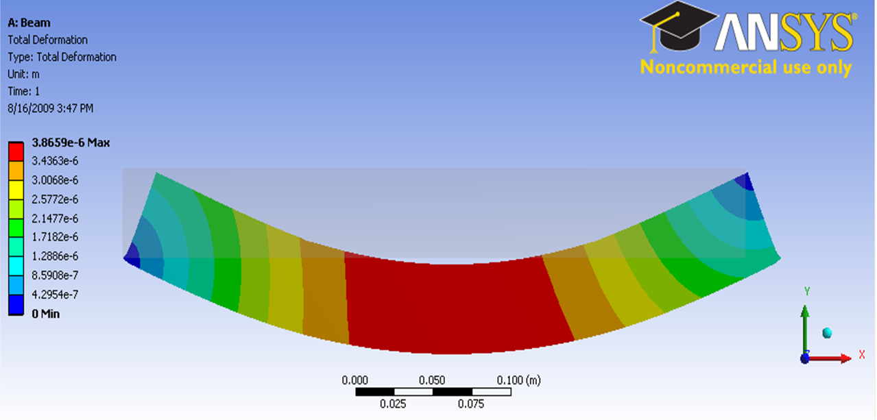
Total Deformation
Let first look at Total Deformation. Under Solution (A6), click on Total Deformation. The Total Deformation plot is then shown in the Graphics window.

Note: To show the original undeformed beam, go to third menu click  and click on
Notice the deformation is exaggerated, revealing that deformation is caused by bending.
You can also animate the deformation by clicking play button right under Graphics window.
Bending Stress
Now let's look at the stress on the beam. Left clicking on User Defined Result under Solution (A6). In the Graphics window show the crank stress contour.

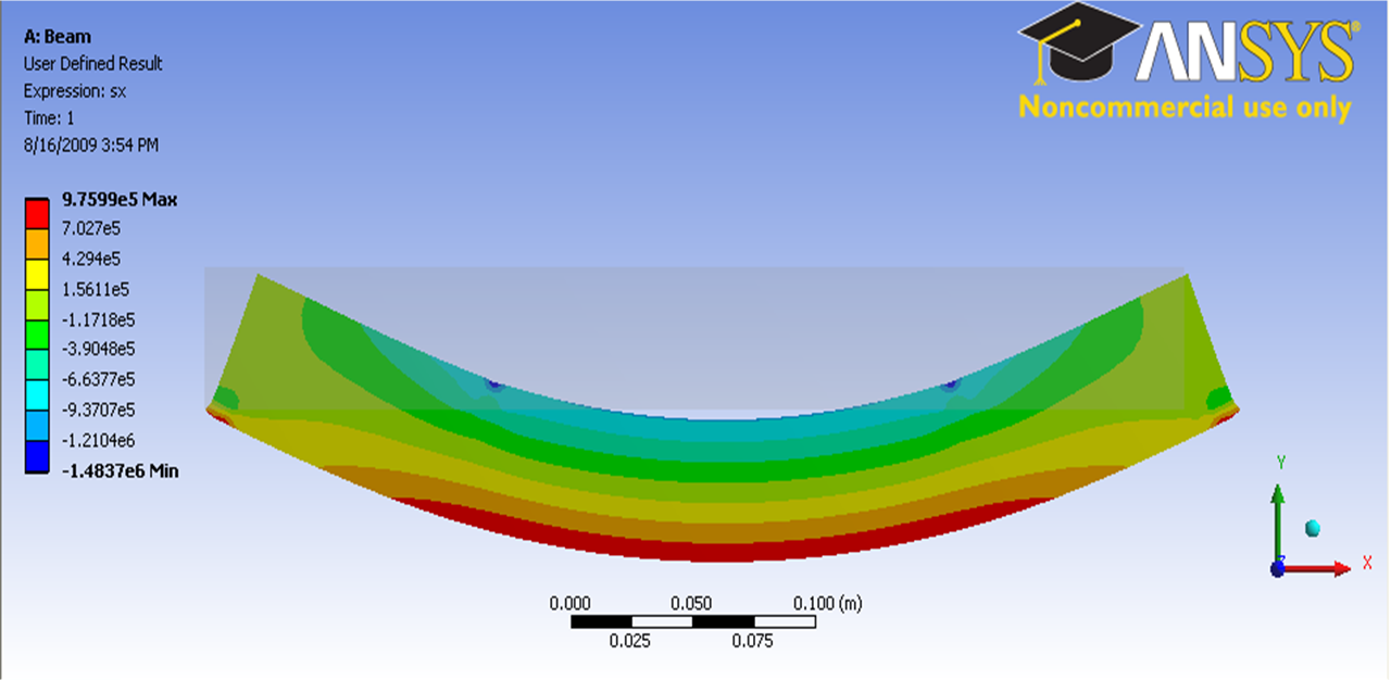
We expect a pure bending stress in the central region between the two applied forces. The stress is tensile on the bottom surface and compressive on the top surface as expected. Elementary beam theory predicts the bending stress as σxx =My/I. Here
M = 4000*0.1 = 400 N m
I =bh3/12 =(1)*(0.05)3/12 = 1.04e-5 m4 (assuming unit thickness in the z direction)
For this geometry, we expect the neutral axis to be at y =h/2 =0.025 m. So the max value of σxx= M*(h/2)/I = 9.6e5 Pa. This is reasonably close to both the maximum value of tensile and compressive stresses from the computational solution. We have a relatively stubby beam; the agreement with beam theory should improve as the length/height ratio of the beam is increased. Also, the FEA solution perhaps can be made more accurate by refining the mesh. This is left as an exercise to the reader.
Note: We see stress concentration appears around the region of the point force and point displacement. A force and displacement applied to a vertex is not realistic and loads to singular stresses (that is , stresses that approach infinity near the loaded vertex). We should disregard stress values in the vicinity of the loaded points.
Go to Step 7: Verification & Validation
Author: Rajesh Bhaskaran & Yong Sheng Khoo, Cornell University
Problem Specification
1. Pre-Analysis & Start-Up
2. Geometry
3. Mesh
4. Setup (Physics)
5. Solution
6. Results
7. Verification & Validation
Step 7: Verification & Validation
It is very important that you take the time to check the validity of your solution. This section leads you through some of the steps you can take to validate your solution.
Simple Checks
Does the bending stress agree with the theoretical value? We checked this in step 6.
Refine Mesh
Let's repeat the solution on a finer mesh with smaller element size. Repeat the mesh steps, but this time we have one additional step after inserting the mapped face mesh. Under Details of "Mesh", expand Defaults and enter value of 100 for Relevance. Click Solve to obtain a new solution.

How does the refined mesh compare with the original mesh?