 Sign-up for free online course on ANSYS simulations!
Step 6: Analyze Results
Plot Velocity Vectors
Let's see the velocity vectors along the airfoil.
Display > Vectors
Enter 4 next to Scale. Enter 3 next to Skip. Click Display.


As can be seen, the velocity of the upper surface is faster than the velocity on the lower surface.
White Background on Graphics Window
To get white background go to:
Main Menu > File > Hardcopy
Make sure that Reverse Foreground/Background is checked and select Color in Coloring section. Click Preview. Click No when prompted "Reset graphics window?"

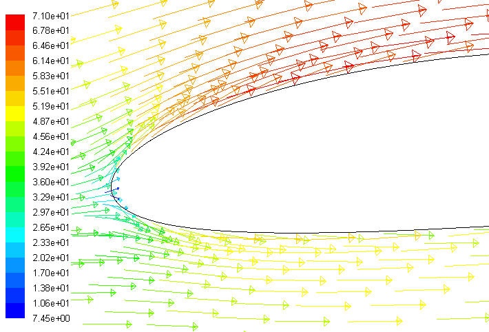
On the leading edge, we see a stagnation point where the velocity of the flow is nearly zero. The fluid accelerates on the upper surface as can be seen from the change in colors of the vectors.

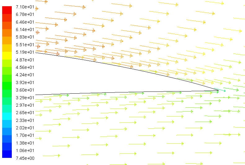
On the trailing edge, the flow on the upper surface decelerates and converge with the flow on the lower surface.
Do note that the time for fluid to travel top and bottom surface of the airfoil is not necessarily the same, as common misconception
Plot Pressure Coefficient
Pressure Coefficient is a dimensionless parameter defined by the equation
Unknown macro: {latex}
\large
$$
Unknown macro: {C_p}
= {{(p-p_
Unknown macro: {ref}
)} \over q_{ref}}
$$
where p is the static pressure,
Pref is the reference pressure, and
qref is the reference dynamic pressure defined by
Unknown macro: {latex}
\large
$$
q_
Unknown macro: {ref}
=
Unknown macro: {1 over 2}
\rho_
{v_{ref}}^2
$$
The reference pressure, density, and velocity are defined in the Reference Values panel in Step 5. Please refer to FLUENT's help for more information. Go to Help > User's Guide Index for help.
Plot > XY Plot...
Change the Y Axis Function to Pressure..., followed by Pressure Coefficient. Then, select airfoil under Surfaces.

Click Plot.

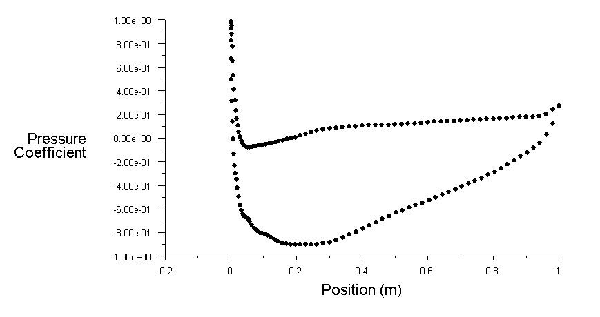
The lower curve is the upper surface of the airfoil and have a negative pressure coefficient as the pressure is lower than the reference pressure.
Plot Pressure Contours
Plot static pressure contours.
Display > Contours...
Select Pressure... and Pressure Coefficient from under Contours Of. Check the Filled and Draw Grid under Options menu. Set Levels to 50. Click Display.


Higher Resolution Image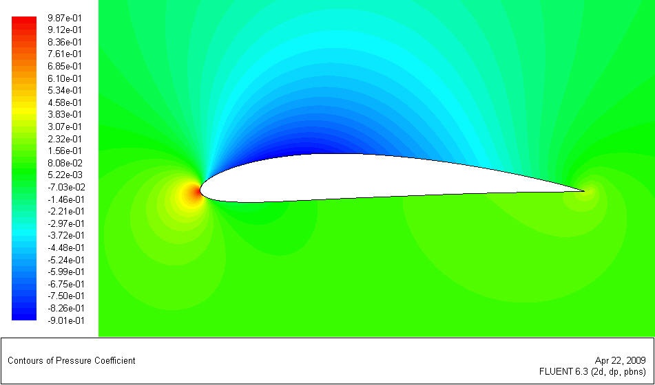
From the figure, we see that in one grid, there is no more than 3 different pressure contours which suggests that our mesh is fine enough.
How can we compare the pressure contour with velocity vector plot? We see that the pressure on the upper surface is negative while the velocity on the upper surface is higher than the reference velocity. Whenever there is high velocity vectors, we have low pressures and vise versa. The phenomenon that we see comply with the Bernoulli equation.
Comparisons
With our simulation data, we can now compare the Fluent with experimental data. The summary of result is shown in the table.
|
CL |
Cd |
FLUENT |
0.647 |
0.00249 |
Experiment |
0.6 |
0.007 |
Theory |
- |
0 |
The experimental data is taken from Theory of Wing Sections By Ira Herbert Abbott, Albert Edward Von Doenhoff pg. 493
Google scholar link
Go to Step 7: Refine Mesh