Page History

...

Pressure Coefficient is a dimensionless parameter defined by the equationwhere equation

Image Added

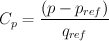
where p is the static pressure, P_ref is the reference pressure, and q_ref is the reference dynamic pressure defined by 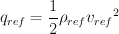Image Added

The appropriate reference values for this problem are the freestream values. byThe reference pressure, density, and velocity are defined in the Reference Values panel in Step 5.
Let's set the reference values necessary to calculate the pressure coefficient.

...

Select pressure-farfield under Compute From.

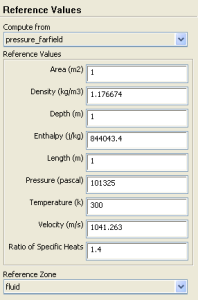
The above This fills in the values from the farfield boundary into this panel. These reference values of density, velocity and pressure will be used to calculate the pressure coefficient from the pressure.

...

The pressure coefficient after the shockwave is 0.293, very close to the theoretical value of 0.289. The pressure increases after the shockwave as we would expect.

Pressure Coefficient Along Wedge

Let's Now we will plot the pressure coefficient along the wedge. Go to:

...

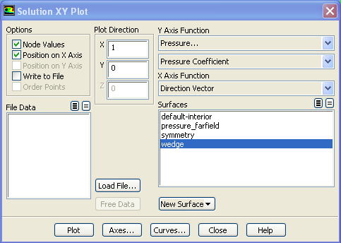
Select XY Plot and then click on the Set up button. In the pop-up window specify the Y Axis Function to pressure and pressure coefficient. Select the wedge from the available surfaces and click Plot.Your specifications should look like the picture below.

The picture above, though descriptive might not give you the details you are looking forIn order to get the values to compare with the analytical solution, it is better to write this data to a file rather than try to read it off the plot. You can save the data used in this plot to a file by checking the Write to File checkbox under  Options. Then click the Write... button, give the file a name and click Function.

To measure the Shock Angle we can add a new line to the plot corresponding to the pressure coefficient at, say, y=0.35m. Click on New Surface and select the Line/Rakeoption. Set the first point to (0,0.35) and the second one to (1.5,0.35) name the line y=0.35 and click on Create.

...

The new line will be added to the available surfaces. From these select Symmetry, Wedge and y=0.35. You will notice that there is no Plot button, this happened because the Write to file checkbox under options is still checked. Uncheck it and then click on Plot. You will now be able to see the lines on the plot.plot. You should be able to calculate the x-location of the shock at y=0.35 from this plot and from that back out the shock angle approximately.

Total Pressure

NextNest, we will plot the Total Pressure. To achieve this on On the Solution XY Plot pop-up window, select Total Pressure under Y Axis Function and click Plot.

Drag Coefficient

Finally, we will find out what the drag coefficient is. FLUENT will integrate the pressure over the wedge to find the net force on the wedge. We'll ask it to take the component in the x-direction to get the drag. This needs to be non-dimensionalized using the appropriate reference values, so we have to set these.

 Close for this scenario is. Close the pop-up window if it's still open and go to

Problem Setup > Reference Values

The reference values of density and velocity were already specified above. Make sure that the parameter entry for Area is 1.  FLUENT uses this as the length scale in calculating the drag coefficient (it doesn't make a distinction between 2D and 3D ... a bit sloppy IMHO). Then go to

Results > Reports > Forces > Set up... > Print

The drag coefficient should be the value listed in the last column of the values in the output window. (The analytical procedure to calculate the drag coefficient is given in Anderson, example 4.9).

Go to Step 7. Verification

...