 Sign-up for free online course on ANSYS simulations!
| Panel |
|---|
| Wiki Markup |
| {alias:flatplate2}
{panel}
Author: Rajesh Bhaskaran, Cornell University {color:#ff0000}{*}Problem Specification{*}{color} [1. Create Geometry in GAMBIT|FLUENT - Forced Convection over a Flat Plate step 1] [2. Mesh Geometry in GAMBIT|FLUENT - Forced Convection over a Flat Plate step 2] [3. Specify Boundary Types in GAMBIT|FLUENT - Forced Convection over a Flat Plate step 3] [4. Set Up Problem in FLUENT|FLUENT - Forced Convection over a Flat Plate step 4] [5. Solve|FLUENT - Forced Convection over a Flat Plate step 5] [6. Analyze Results|FLUENT - Forced Convection over a Flat Plate step 6] [7. Refine Mesh|FLUENT - Forced Convection over a Flat Plate step 7] {panel} h2. Problem Specification !daplate.jpg! In our problem, we have a flat plate at a constant temperature of 413K. The plate is infinitely wide. The velocity profile of the fluid is uniform at the point x = 0. The free stream temperature of the fluid is 353K. The assumption of incompressible flow becomes invalid increasingly less valid for larger temperature differences between the plate and freestream. Because of this, we will treat this as a compressible flow. We will analyze a fluid flow with the following non-dimensional conditions: !Re_Pr.jpg! In order to achieve these flow conditions, we will use these free stream flow conditions: !01_properties.jpg! According to the ideal gas law, this temperature and pressure result in the following freestream density: !01_density.jpg! These flow conditions do not necessarily represent a realistic fluid. Rather, they are chosen to provide the Prandtl and Reynolds numbers specified above. This will make calculations simpler throughout this tutorial. Solve this problem in FLUENT. Validate the solution by plotting the y\+ values at the plate. Also plot the velocity profile at x = 1m. Then plot Reynolds Number vs. Nusselt Number. Compare the accuracy of your results from FLUENT with empirical correlations. h4. Preliminary Analysis We expect the turbulent boundary layer to grow along the plate. As the boundary layer grows in thickness, the rate of heat transfer (q'') and thus the heat transfer coefficient (h) will decrease. !00fp2.jpg! We will compare the numerical results with experimentally-derived heat transfer correlations. We will create the geometry and mesh in GAMBIT, read the mesh into FLUENT, and solve the flow problem. Go to Step [1: Create Geometry in GAMBIT|FLUENT - Forced Convection over a Flat Plate step 1] [See and rate the complete Learning Module|FLUENT - Forced Convection over a Flat Plate] Go to [all FLUENT Learning Modules|FLUENT Learning Modules]University Problem Specification |
Problem Specification
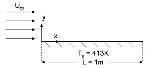
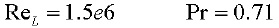
In our problem, we have a flat plate at a constant temperature of 413K. The plate is infinitely wide. The velocity profile of the fluid is uniform at the point x = 0. The free stream temperature of the fluid is 353K. The assumption of incompressible flow becomes invalid increasingly less valid for larger temperature differences between the plate and freestream. Because of this, we will treat this as a compressible flow. We will analyze a fluid flow with the following non-dimensional conditions:
In order to achieve these flow conditions, we will use these free stream flow conditions:
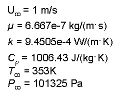
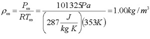
According to the ideal gas law, this temperature and pressure result in the following freestream density:
These flow conditions do not necessarily represent a realistic fluid. Rather, they are chosen to provide the Prandtl and Reynolds numbers specified above. This will make calculations simpler throughout this tutorial.
Solve this problem in FLUENT. Validate the solution by plotting the y+ values at the plate. Also plot the velocity profile at x = 1m. Then plot Reynolds Number vs. Nusselt Number. Compare the accuracy of your results from FLUENT with empirical correlations.
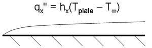
Preliminary Analysis
We expect the turbulent boundary layer to grow along the plate. As the boundary layer grows in thickness, the rate of heat transfer (q'') and thus the heat transfer coefficient (h) will decrease.
We will compare the numerical results with experimentally-derived heat transfer correlations. We will create the geometry and mesh in GAMBIT, read the mesh into FLUENT, and solve the flow problem.
Go to Step 1: Create Geometry in GAMBIT