 Sign-up for free online course on ANSYS simulations!
Step 4: Set Up Problem in FLUENT
Launch Fluent 6.0
Start > Programs > Fluent Inc > FLUENT 6.0
Select the 2ddp version and click Run.
The "2ddp" option is used to select the 2-dimensional, double-precision solver. In the double-precision solver, each floating point number is represented using 64 bits in contrast to the single-precision solver which uses 32 bits. The extra bits increase not only the precision but also the range of magnitudes that can be represented. The downside of using double precision is that it requires more memory. |
Import Grid
Main Menu > File > Read > Case...
Navigate to the working directory and select the plate.msh file. This is the mesh file that was created using the preprocessor GAMBIT in the previous step. FLUENT reports the mesh statistics as it reads in the mesh:

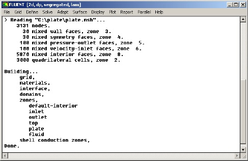
Check the number of nodes, faces (of different types) and cells. There are 3000 quadrilateral cells in this case. This is what we expect because we used 30 divisions in the horizontal direction and 100 divisions in the vertical direction while generating the grid. So the total number of cells is 30*100 = 3000.
Also, take a look under zones. We can see the four zones inflow, outflow, top, and plate that we defined in GAMBIT.
Check and Display Grid
First, we check the grid to make sure that there are no errors.
Main Menu > Grid > Check
Any errors in the grid would be reported at this time. Check the output and make sure that there are no errors reported. Check the grid size:
Main Menu > Grid > Info > Size
The following statistics should appear:

Display the grid:
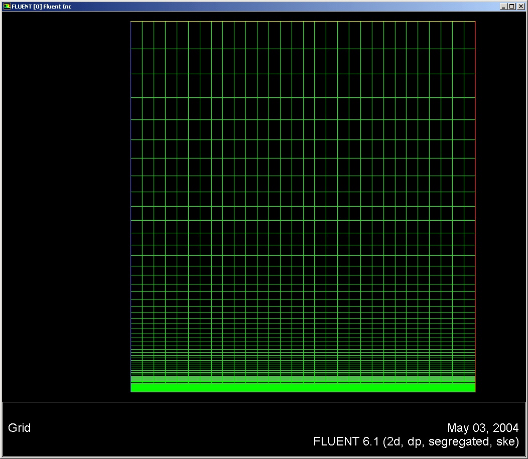
Main Menu > Display > Grid...
Make sure all 5 items under Surfaces are selected.

Then click Display. The graphics window opens and the grid is displayed in it. Your grid should look like this:

Define Solver Properties
Main Menu > Define > Models > Solver
We'll use the defaults of 2D space, segregated solver, implicit formulation, steady flow and absolute velocity formulation. Click OK.

Main Menu > Define > Models > Energy
We are interested in solving the temperature distribution, so we need to solve the energy equation. Select the Energy Equation and click OK to exit the menu.

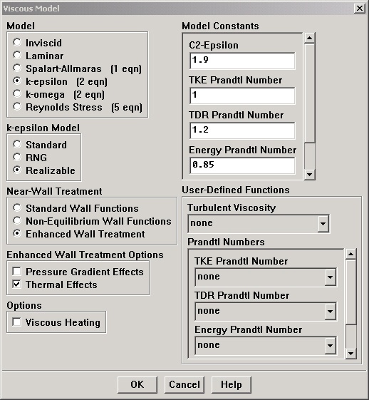
Main Menu > Define > Models > Viscous
Under Model, select the k-epsilon turbulence model. We will use the Realizable model in the k-epsilon Model box. The Realizable k-epsilon model produces more accurate results for boundary layer flows than the Standard k-epsilon model. In the Near-Wall Treatment box, observe the Enhanced Wall Treatment option, which deals with the resolution of the boundar layer in our model. There are 3 regions in the boundary layer that we are concerned with, starting at the wall:
1. Laminar sublayer (y+ < 5)
2. Buffer region (5 < y+ < 30)
3. Turbulent region (y+ > 30)
y+ is a mesh-dependent dimensionless distance that quantifies to what degree the wall layer is resolved. After solving this problem in FLUENT, we will observe the value of y+ for each mesh we use. The Enhanced Wall Treatment option serves to more accurately resolve the boundary layer in the case when the mesh is only fine enough to resolve to the turbulent region (y+ > 30). Enhanced Wall Treatment also improves the accuracy of meshes that can only be resolved to the Buffer region (5< y+ < 30). However, solutions with y+ values in the buffer region are generally less accurate than if the solution is resolved to one of the other 2 regions. Look at FLUENT Help section 10.9, Grid Considerations for Turbulent Flow Simulations, for more details.
For our mesh, FLUENT will be able to resolve the laminar sublayer, thus Enhanced Wall Treatment does not improve the accuracy of our solution with our mesh. It will however make a difference in Step 7 when we use a less refined mesh. The thickness of the boundary layer is significantly smaller than the height of our flow field. Resolving the solution to the laminar sublayer is computationally intensive, especially in high Reynolds Number flows. Resolving to the turbulent region is often the only reasonable option. Thus it is good practice to always use Enhanced Wall Treatment when dealing with a boundary layer. Although it is not necessary with the current mesh, it will be necessary for the less refined mesh later on, so go ahead and select Enhanced Wall Treatment now.
Select Thermal Effects in the Enhanced Wall Treatment Options box to include the thermal terms in the Enhanced Wall Treatment equation.
The values in the Model Constants box are constants used in the k-epsilon turbulence equations. These values for the Model Constants are well-accepted for a wide range of wall-bounded shear flows. Leave all values in the Model Constants box set to their default values.
Click OK.

Define Material Properties
Main Menu > Define > Materials...
Change Density to ideal gas because we are treating the flow as compressible. FLUENT will calcualte the density of the flow at each point based on the pressure and temperature it calculates at that point. Leave Cp set as the default value of 1006.43. Change Thermal Conductivity to 9.4505 e-4. Change Viscosity to 6.667e-7. Scroll down to see Molecular Weight. Leave Molecular Weight set to the default value of 28.966. These are the values that we specified under Problem Specification.

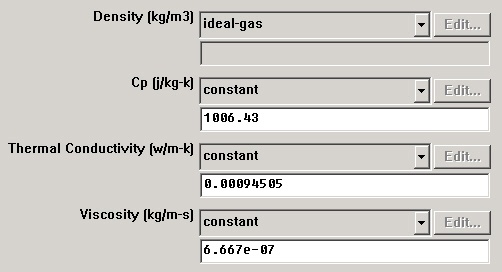
Click Change/Create. Simply clicking close without clicking Change/Create will cause these properties to revert back to their default values.
Define Operating Conditions
Main Menu > Define > Operating Conditions...
For all flows, FLUENT uses gauge pressure internally. Any time an absolute pressure is needed, it is generated by adding the operating pressure to the gauge pressure. We'll use the default value of 1 atm (101,325 Pa) as the Operating Pressure.
Click Cancel to leave the default value in place.

Define Boundary Conditions
We'll now set the value of the velocity at the inflow and pressure at the outflow.
Main Menu > Define > Boundary Conditions...
We note here that the four types of boundaries we defined are specified as zones on the left side of the Boundary Conditions Window. There are also 2 zones default-interior fluid, used to define the interior of the flow field. We will not need to change any setting for these 2 zones.
Move down the list and select inflow under Zone. Note that FLUENT indicates that the Type of this boundary is velocity-inlet. Recall that the boundary type for the inflow was set in GAMBIT. If necessary, we can change the boundary type set previously in GAMBIT in this menu by selecting a different type from the list on the right. Click Set....
Enter 1 for Velocity Magnitude. This sets the velocity of the fluid entering at the left boundary to a uniform velocity profile of 1m/s. Set Temperature to 353K. Change Turbulence Specification Method to Intensity and Viscosity Ratio. Set Turbulence Intensity to 1 and Turbulent Viscosity Ratio to 1. Click OK.


Choose outflow under Zone. The Type of this boundary is pressure-outlet. Click Set.... The default value of the Gauge Pressure is 0. The (absolute) pressure at the outflow is 1 atm. Since the operating pressure is set to 1 atm, the outflow gauge pressure = outflow absolute pressure - operating pressure = 0. Because we do not expect any backflow, we do not need to set any backflow conditions. Click Cancel to leave the defaults in place.


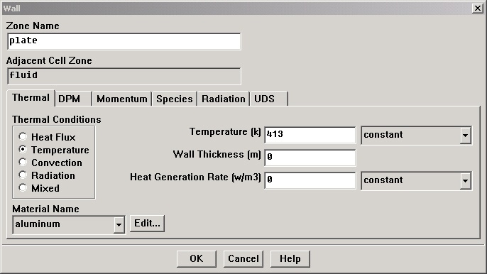
Click on plate under Zones and make sure Type is set as wall. Click Set.... Because we have a heated isothermal plate, we need to set the temperature. On the Thermal tab, select Temperature under Thermal Conditions. Change Temperatureto 413. The material selected is inconsequential because the plate has zero thickness in our model, thus the material properties of the plate do not affect the heat transfer properties of the plate. Click OK.

The last boundary condition to set is for the top of the flow field. Click on top under Zones and make sure Type is set as symmetry. Click Set... to see that there is nothing to set for this boundary. Click OK.
Click Close to close the Boundary Conditions menu.
Go to Step 5: Solve!