 Sign-up for free online course on ANSYS simulations!
Step 7: Refine Mesh
It is very important to assess the dependence of your results on the mesh used by repeating the same calculation on different meshes and comparing the results. We will re-do the previous calculation on a 30 x 50 mesh as well as a 30 x 150 mesh and then compare the results with the 30x100 mesh used previously.
Modify Mesh in GAMBIT to a 30x50 mesh
The 30x100 mesh is saved as plate.dbs in your working directory. Bring up the command prompt window as in step 1. To copy plate.dbs to plate50.dbs, at the command prompt, type
copy plate.dbs plate50.dbs
We will work with plate50.dbs in order to retain plate.dbs as is. Launch GAMBIT with plate50.dbs as the input file by typing:
gambit plate50.dbs
Follow the same method as in previous tutorials to change the mesh. The face mesh will be automatically deleted when you re-mesh the edges. The top and bottom edges will remain the same.
Mesh the inflow and outflow edges at a Successive Ratio of 1.095 and an Interval Count of 50.

Remesh the face and then export this as the 2D mesh file, plate50.msh.
Read the file into FLUENT and repeat step 4 and step 5 of this tutorial to set up and solve the problem in FLUENT. The solution should converge in approximately 115 iterations. Plot y+ at the plate as explained in step 6.

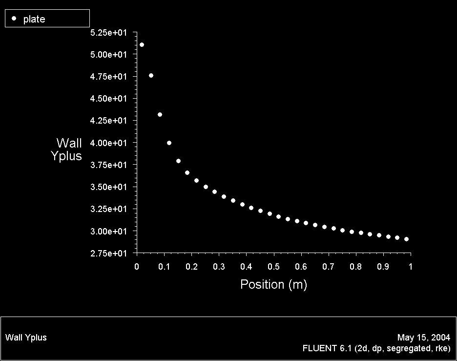
y+ ranges from 29 to 50 in this plot. This is (mostly) outside of the ill-defined Buffer region (5 < y+ < 30) and is thus acceptable.
Now use the Total Surface Heat Flux plot to determine Nux . Plot Re vs. Nu and compare with the 30x100 mesh results.

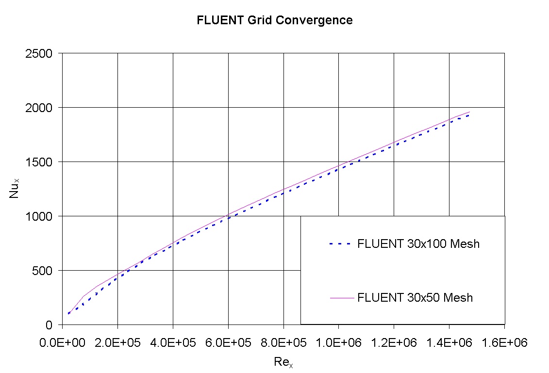
We can see that the courser mesh produces slightly different results, although they are still reasonable. Some numerical error is introduced when the less-refined 30x50 mesh is used. As one would expect, resolving the boundary layer to the laminar sublayer, which we did with the orignial mesh, produces more accurate results than resolving only to the turbulent region. Resolving to the laminar sublayer is not always a reasonable thing to do, especially at high Reynolds numbers. The results from using the 30 x 50 grid show that a reasonable solution can still be obtained without resolving down to the laminar sublayer.
Modify Mesh in GAMBIT to a 30x150 mesh
Create a mesh that is finer than the original mesh to see if our original solution contained inaccuracies due to the mesh. Mesh the inflow and outflow edges at a Successive Ratio of 1.065 and an Interval Count of 150.

Remesh the face and then export this as the 2D mesh file, plate150.msh.
Read the file into FLUENT and repeat step 4 and step 5 of this tutorial to set up and solve the problem in FLUENT. The solution should converge in approximately 4550 iterations. Plot y+ at the plate.

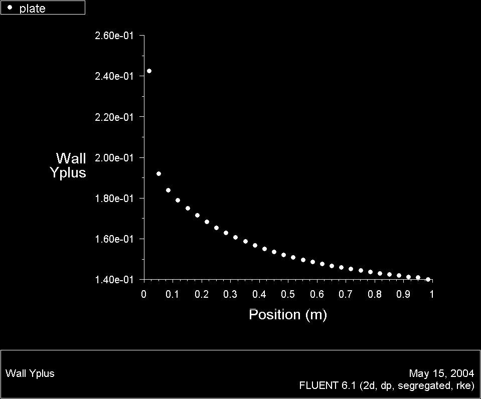
y+ ranges from 0.14 to 0.25 in this plot, well within the laminar sublayer.
Now use the Total Surface Heat Flux plot to determine Nux . Plot Re vs. Nu and compare with the 30x100 mesh results.

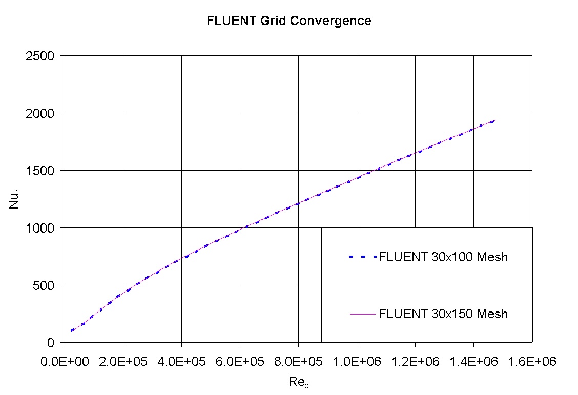
This plot shows that the results did not change by increasing the fineness of the mesh. Thus, we can conclude that our 30x100 mesh was good enough. It is also important to verify that the solution does not change by refining the mesh in the streamwise direction. In this case, the mesh in the streamwise direction is already fine enough to eliminate mesh-dependent numerical error.