Pre-Analysis and Start-Up

Analytical vs. Numerical Approaches

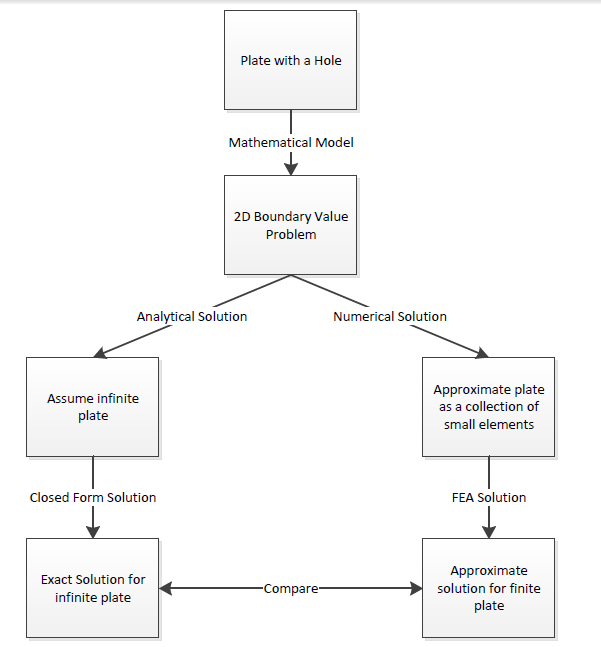
We can either assume the geometry as an infinite plate and solve the problem analytically, or approximate the geometry as a collection of "finite elements", and solve the problem numerically. The following flow chart compares the two approaches.

Let's first review the analytical results for the infinite plate. We'll then use these results to check the numerical solution from ANSYS.

Analytical Results

Displacement

Let's estimate the expected displacement of the right edge relative to the center of the hole. We can get a reasonable estimate by neglecting the hole and approximating the entire plate as being in uniaxial tension. Dividing the applied tensile stress by the Young's modulus gives the uniform strain in the x direction.

Multiplying this by the half-width (5 in) gives the expected displacement of the right edge as ~ 0.1724 in. We'll check this against ANSYS.

Sigma-r

Let's consider the expected trends for Sigma-r, the radial stress, in the vicinity of the hole and far from the hole. The analytical solution for Sigma-r in an infinite plate is:

where a is the hole radius and Sigma-o is the applied uniform stress (denoted P in the problem specification). At the hole (r=a), this reduces to

This result can be understood by looking at a vanishingly small element at the hole as shown schematically below.

We see that Sigma-r at the hole is the normal stress at the hole. Since the hole is a free surface, this has to be zero.

For r>>a,

Far from the hole, Sigma-r is a function of theta only. At theta = 0, Sigma-r ~ Sigma-o. This makes sense since r is aligned with x when theta = 0. At theta = 90 deg., Sigma-r ~ 0 which also makes sense since r is now aligned with y. We'll check these trends in the ANSYS results.

Sigma-theta

Let's next consider the expected trends for Sigma-theta, the circumferential stress, in the vicinity of the hole and far from the hole. The analytical solution for Sigma-theta in an infinite plate is:

At r = a, this reduces to

At theta = 90 deg., Sigma-theta = 3*Sigma-o for an infinite plate. This leads to a stress concentration factor of 3 for an infinite plate.

For r>>a,

At theta = 0 and theta = 90 deg., we get

Far from the hole, Sigma-theta is a function of theta only but its variation is the opposite of Sigma-r (which is not surprising since r and theta are orthogonal coordinates; when r is aligned with x, theta is aligned with y and vice-versa). As one goes around the hole from theta = 0 to theta = 90 deg., Sigma-theta increases from 0 to Sigma-o. More trends to check in the ANSYS results!

Tau-r-theta

The analytical solution for the shear stress Tau-r-theta in an infinite plate is:

At r=a,

By looking at a vanishingly small element at the hole , we see that Tau-r-theta is the shear stress on a stress surface, so it has to be zero.

For r>>a,

We can deduce that, far from the hole, Tau-r-theta = 0 both at theta = 0 and theta = 90 deg. Even more trends to check in ANSYS!

Sigma-x

First, let's begin by finding the average stress, the nominal area stress, and the maximum stress with a concentration factor.

The concentration factor for an infinite plate with a hole is K = 3. The maximum stress for an infinite plate with a hole is

Although there is no analytical solution for a finite plate with a hole, there is empirical data available to find a concentration factor. Using a Concentration Factor Chart (Cornell 3250 Students: See Figure 4.22 on page 158 in Deformable Bodies and Their Material Behavior), we find that d/w = 1 and thus K ~ 2:73 Now we can find the maximum stress using the nominal stress and the concentration factor

Open ANSYS Workbench

Now that we have the pre-calculations, we are ready to do a simulation in ANSYS Workbench! Open ANSYS Workbench by going to Start > ANSYS > Workbench. This will open the start up screen as seen below

To begin, we need to tell ANSYS what kind of simulation we are doing. If you look to the left of the start up window, you will see the Toolbox Window. Take a look through the different selections. The plate with a hole is a static structural simulation. Load the static structural tool box by dragging and dropping it into the Project Schematic.

Name the Project "Plate with a Hole" by double clicking the text Static Structural and typing in Plate with a Hole.

Material Selection

Now we need to specify what type of material we are working with. Double click Engineering Data and it will take you to the Engineering Data Menus.

If you look under the Outline of Schematic A2: Engineering Data Window, you will see that the default material is Structural Steel. The Problem Specification specifies the material's Modulus of Elasticity and Poisson's ratio. To add a new material, click in an empty box labeled Click here to add a new material and give it a name. We will call our material Cornellium.

On the left hand side of the screen in the Toolbox window, expand Linear Elastic and double click Isotropic Elasticity to specify the Elastic Modulus and Poisson's Ratio.

In the Properties of Outline Row 4: Cornellium window, Set the Elastic Modulus units to psi, set the magnitude as 29e6, and set the Poisson's Ratio to .3.

Close the materials window by selecting Return to Project.

Now that the material has been specified, we are ready to make the geometry in ANSYS.

Go to Step 2: Geometry

Go to all ANSYS Learning Modules