Turbulent Jet Setup and Solution

Background

The k-ε model solves the RANS - Reynolds Averaged Navier Stokes model, which solves time-averaged Navier Stokes equations.Two additional equations for the turbulent kinetic energy k, and the turbulent dissipation ε, account for the turbulent properties, using the turbulent viscosity to calculate the additional Reynolds stress terms that emerge when time averaging the Navier Stokes equations. It is one of the more widely used models, particularly for flows with small pressure gradients. 

The following empirical formulas are useful in defining this model. I is the turbulent intensity,

 is the hydraulic diameter, and d is the jet diameter. 

,   

,  

,  

Setup

Use the same case and data files as you downloaded in the Laminar setup for the geometry and mesh. 

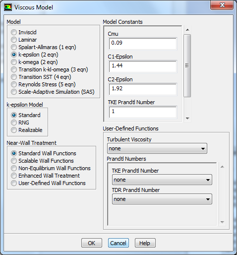
Now, set up the k-ε model for turbulence. In Solution Setup-Models, double click the previous "Viscous-Laminar" option to open the dialogue. Select the "k-epsilon (2eqn)" model for turbulence. Leave the model constants the same as defined in the dialogue below; these values have been refined to constraints of the model and are typically not varied. Press OK.

 
In the Materials dialogue. change the viscosity for a higher Reynolds number:

The inlet jet velocity will remain at 1m/s; the inlet diameter is still 0.01m from the geometry (ignoring the larger diameter with 0m/s velocity inflow), so enter the viscosity for air as ν = 1E-7. Select Change/Create and then Close.

The k-ε terms must be specified on all boundaries. Go to Solution Setup - Boundary Conditions and edit both Farfield and Inlet boundaries. Select "Intensity and Hydraulic Diameter" as the turbulence specification method. At Inlet 1, from the specified Reynolds number and above equations, the intensity should be I=0.037942, and the hydraulic diameter should be 0.01m (twice the measured inlet height).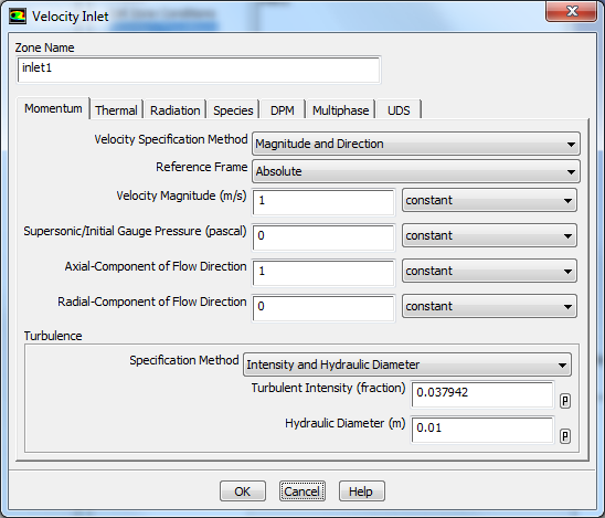 

The other Inlet and both Farfield boundaries should have turbulent kinetic energy and dissipation rates set to zero, because there is no inlet velocity or turbulence associated with them. Press OK for all boundaries to save the inputs.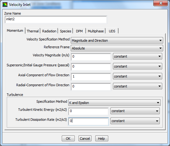
To initialize the solution, go to Solution Initialization. Select "Inlet 1" to initialize the domain, and press "Initialize". 

To accelerate convergence and just solve the flow equations initially without turbulence, go to Solution - Solution Controls - Equations. Unselect Turbulence and press OK.  

Go to Solution - Run Calculation. Run the calculation for 2000 iterations, monitoring the residuals. Now go back to Solution - Solution Controls - Equations. Select Turbulence and press OK. 

Go to Monitors, select "Residuals" and press Edit. Change the absolute convergence criteria for k and ε to be 1E-06.  Make sure to de-select the Convergence check box for all residual quantities.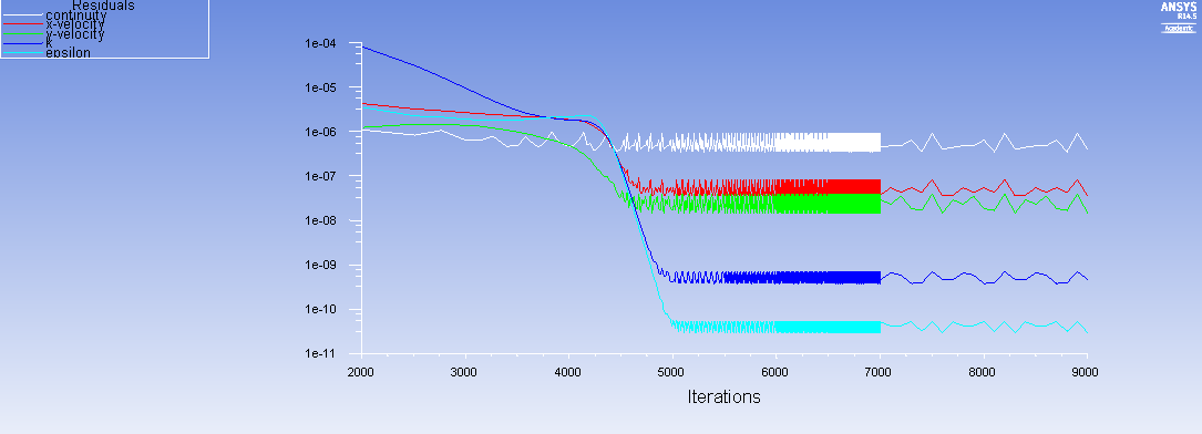
Now go back to Run Calculation. Run the solution until it all residuals appear to reach a steady state value. This should take less than 5000 iterations, and you should end up with a residuals plot somewhat like this:
Export the results to CFD-Post by clicking "File-Export to CFD Post". Select Axial Velocity, Turbulent Kinetic Energy k, Turbulent dissipation ε, Turbulent Intensity I, and X and Y coordinates. Select "Write to CFD Post" and "Open CFD Post" and then click "Write".

Go to Step 5: Turbulent Jet Results

Go to all FLUENT Learning Modules