 Sign-up for free online course on ANSYS simulations!
Unable to render {include} The included page could not be found.
Author: John Singleton and Rajesh Bhaskaran, Cornell University
Problem Specification
1. Pre-Analysis & Start-up
2. Geometry
3. Mesh
4. Setup (Physics)
5. Solution
6. Results
7. Verification & Validation
Exercises
Post Processing
We will use CFD-Post as the primary post processing GUI. Steps for post processing in FLUENT can be found here.
Step 6. Results
Double click on Results from the Workbench Window to launch CFD-Post.
Velocity Vectors
Click on the z-axis,  to view the XY plane. Click on the vector icon to insert a vector plot. Name it Velocity Vector.
A panel named "Details of Velocity Vector" will appear right below the outline window. Set the Locations to symmetry 1. Click on Apply to display the velocity vectors.

The velocity vectors will be displayed in the view window.
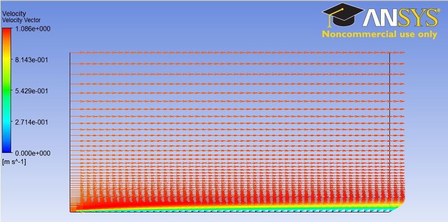
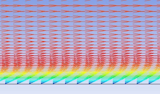
You can use the wheel button of the mouse to zoom into the region that closely surrounds the plate, to get a better view of the boundary layer velocities:
Outlet Velocity Profile
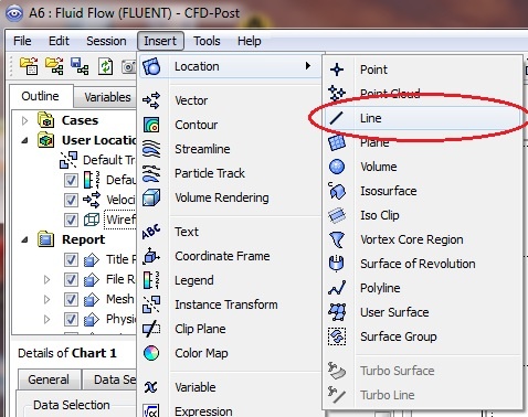
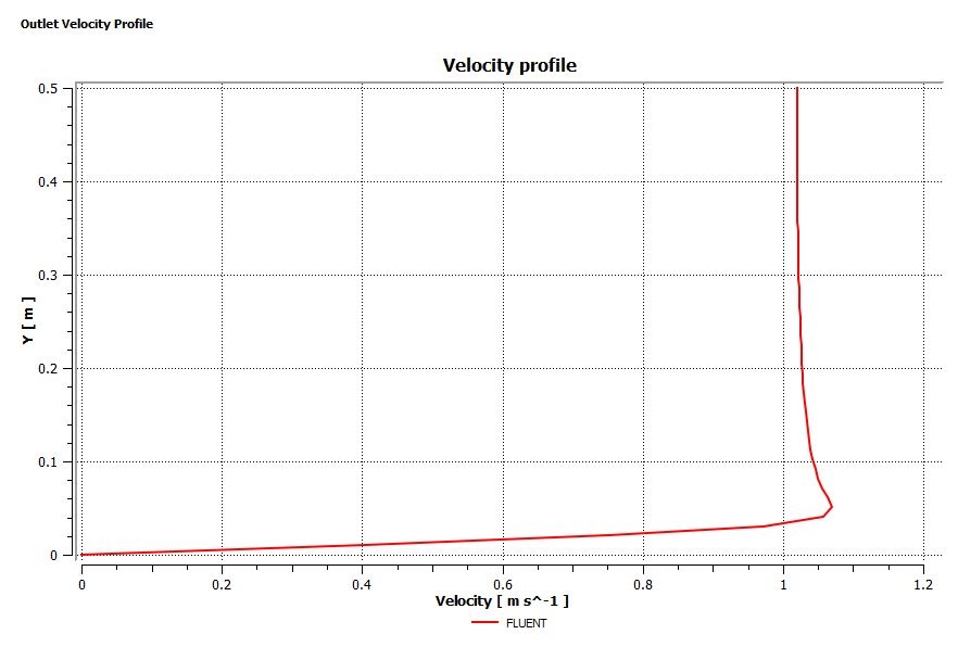
From the menu, insert > location > line. Name it "Outlet"
In the Details of Outlet panel, enter the following coordinates. Change the number of samples to 50. Click on Apply to create a line at the outlet.

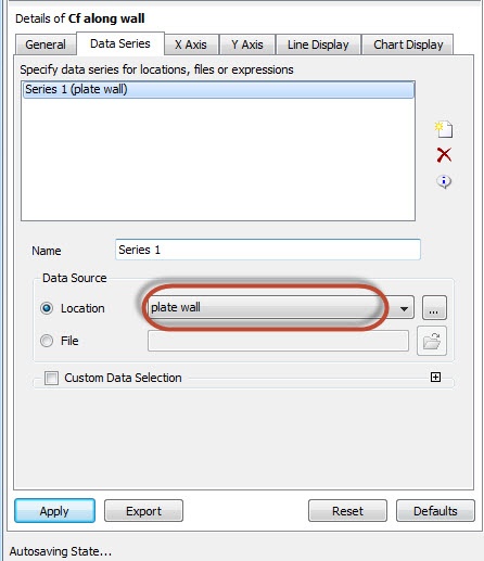
Insert a chart from the menu: insert > chart. Name the chart "Outlet Velocity Profile". Change the title to "Velocity Profile" in the General tab. In the Data Series tab, rename Series 1 to FLUENT and select Outlet for location. Select Velocity as the variable in the X Axis tab and select Y as the variable in the Y Axis tab. Click on Apply to generate the chart.
The velocity profile at the outlet is shown below:
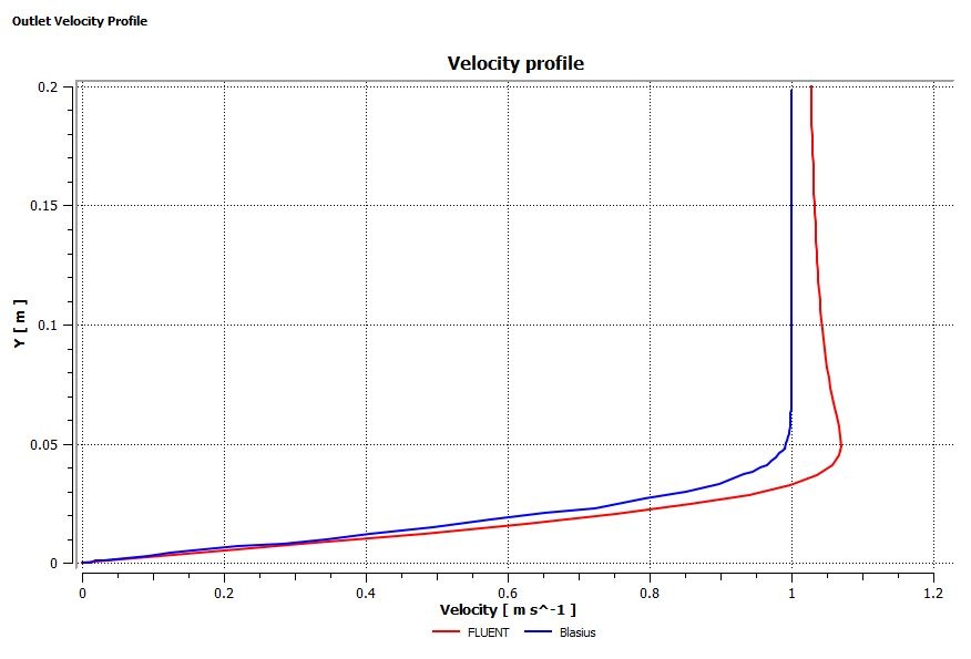
We would like to compare the FLUENT result to the Blasius boundary layer solution. Download the Blasius solution here. Return to the Data Series tab and insert another data set. Rename it Blasius. Instead of specifying the location of the data, select the Blasius solution file you have downloaded.

Click on Apply. The comparison should look like the following plot:
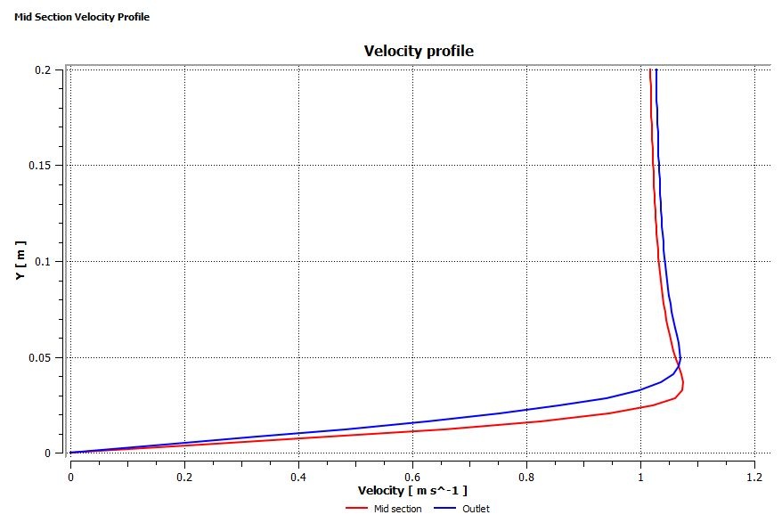
Mid-Section Velocity Profile
Here, we will plot the variation of the x component of the velocity along a vertical line in the middle of the geometry. In order to create the profile, we must first create a vertical line at x=0.5m. Insert another line, same as the previous step, and name it Mid section. Enter the following numbers to create a vertical line at x=0.5m. Set the number of samples to 50. Remember to click on Apply to finish.

Insert another chart and name it Mid Section Velocity Profile. In the General tab, change the title to "Velocity profile". Select Mid Section as the location and rename Series 1 to Mid section. We will compare the velocity profiles at the mid section and at the outlet. Repeat the procedure in the previous step to insert the velocity profile at the outlet. Change the variable to Velocity in the X Axis tab and change the variable to Y in the Y Axis tab. Click on Apply to generate the chart.
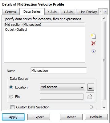
The velocity profile comparison is shown below:
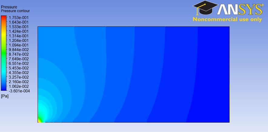
Pressure Contour
Insert > Contour. Name it Pressure contour.
In Details of Pressure contour, change the locations to symmetry 1, change the variable to Pressure, and change the number of contours to 50.
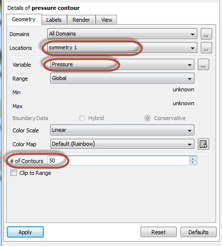
Click on Apply to view the contour.
Go to Step 7: Verification & Validation