Plate With a Hole Tutorial - Pre-Analysis and Start-Up

Analytical vs. Numerical Approaches

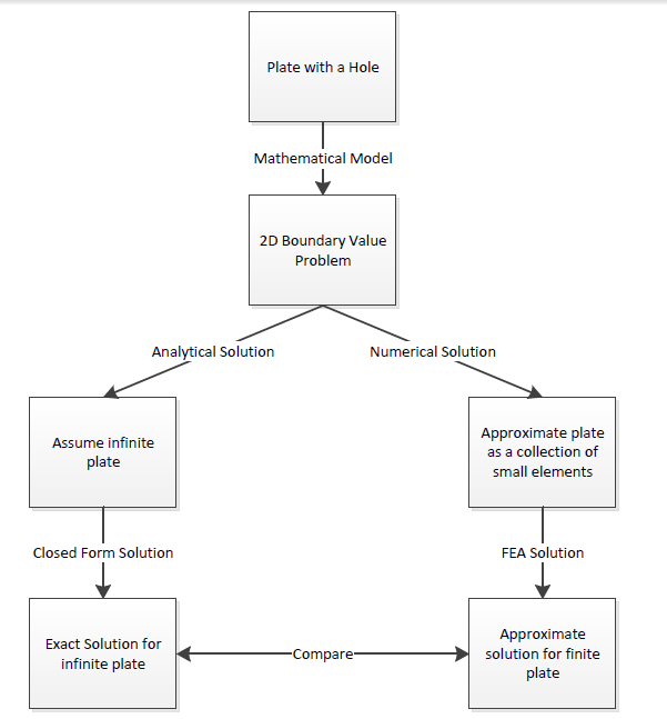
We can either assume the geometry as an infinite plate and solve the problem analytically, or approximate the geometry as a collection of "finite elements", and solve the problem numerically. The following flow chart compares the two approaches.

Click here to enlarge image

Let's first review the analytical results for the infinite plate. We'll then use these results to check the numerical solution from ANSYS.

Analytical Results

Displacement

Let's estimate the expected displacement of the right edge relative to the center of the hole. We can get a reasonable estimate by neglecting the hole and approximating the entire plate as being in uniaxial tension. Dividing the applied tensile stress by the Young's modulus gives the uniform strain in the x direction. Multiplying this by the half-width (5 in) gives the expected displacement of the right edge as ~ 0.17 in. We'll check this against ANSYS.

Sigma-r

Let's consider the expected trends for Sigma-r, the radial stress, in the vicinity of the hole and far from the hole. The analytical solution for Sigma-r in an infinite plate is:

where a is the hole radius and Sigma-o is the applied uniform stress (denoted P in the problem specification). At the hole (r=a), this reduces to

This result can be understood by looking at a vanishingly small element at the hole as shown schematically below.

We see that Sigma-r at the hole is the normal stress at the hole. Since the hole is a free surface, this has to be zero.

For r>>a,

Far from the hole, Sigma-r is a function of theta only. At theta = 0, Sigma-r ~ Sigma-o. This makes sense since r is aligned with x when theta = 0. At theta = 90 deg., Sigma-r ~ 0 which also makes sense since r is now aligned with y. We'll check these trends in the ANSYS results.

Sigma-theta

Let's next consider the expected trends for Sigma-theta, the circumferential stress, in the vicinity of the hole and far from the hole. The analytical solution for Sigma-theta in an infinite plate is:

At r = a, this reduces to

At theta = 90 deg., Sigma-theta = 3*Sigma-o for an infinite plate. This leads to a stress concentration factor of 3 for an infinite plate.

For r>>a,

At theta = 0 and theta = 90 deg., we get

Far from the hole, Sigma-theta is a function of theta only but its variation is the opposite of Sigma-r (which is not surprising since r and theta are orthogonal coordinates; when r is aligned with x, theta is aligned with y and vice-versa). As one goes around the hole from theta = 0 to theta = 90 deg., Sigma-theta increases from 0 to Sigma-o. More trends to check in the ANSYS results!

Tau-r-theta

The analytical solution for the shear stress Tau-r-theta in an infinite plate is:

At r=a,

By looking at a vanishingly small element at the hole , we see that Tau-r-theta at the hole is the shear stress at the hole. Since the hole is a free surface, this has to be zero.

For r>>a,

We can deduce that, far from the hole, Tau-r-theta = 0 both at theta = 0 and theta = 90 deg. Even more trends to check in ANSYS!

ANSYS Simulation

Now, let's load the problem into ANSYS and see how a computer simulation will compare. First, start by downloading the files here

The zip file should contain the following contents:

• Plate With a Hole_files folder
• Plate With a Hole.wbpj

Please make sure to extract both of these files from the zip folder, the program will not work otherwise. (Note: The solution was created using ANSYS workbench 12.1 release, there may be compatibility issues when attempting to open with other versions).

2. Double click "Plate With a Hole.wbpj" - This should automatically open ANSYS workbench (you have to twiddle your thumbs a bit before it opens up). You will be presented with the ANSYS solution.

A tick mark against each step indicates that that step has been completed.

3. To look at the results, double click on "Results" - This should bring up a new window (again you have to twiddle your thumbs a bit before it opens up).

4. On the left-hand side there should be an "Outline" toolbar. Look for "Solution (A6)".

We'll investigate the items listed under Solution in the next step in this tutorial.

Continue to Step 2 - Results
Go to all ANSYS Learning Modules