FLUENT - Flat Plate Boundary Layer - Results

Step 6: Results

Velocity Vectors

One can plot vectors in the entire domain, or on selected surfaces. Here, the vectors will be plotted for the entire domain. First, click on Graphics & Animations . Next, double click on Vectors which is located under Graphics. Then, click on Display in the Vectors menu. You should obtain, the following output.

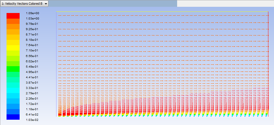
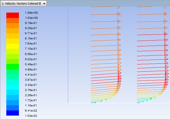
You can use the wheel button of the mouse to zoom into the region that closely surrounds the plate, to get a better view of the boundary layer velocities.

Outlet Velocity Profile

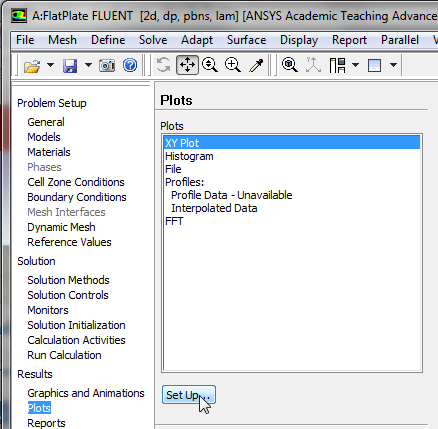
In this section we will first plot the variation of the x component of the velocity along the outlet. Then we will plot the Blasius solution and to see how the numerical solution compares. In order to start the process (Click) Results > Plots > XY Plot... > Set Up.. as shown below.

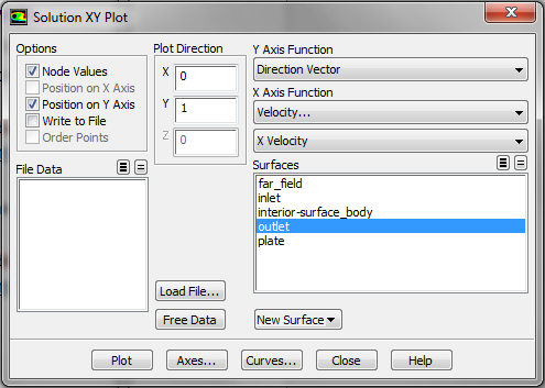
In the Solution XY Plot menu make sure that Position on Y Axis is selected , and X is set to 0 and Y is set to 1. This tells FLUENT to plot the y-coordinate value on the ordinate of the graph. Next, select Velocity... for the first box underneath X Axis Function and select X Velocity for the second box. Please note that X Axis Function and Y Axis Function describe the x and y axes of the graph, which should not be confused with the x and y directions of the geometry. Finally, select outlet under Surfaces since we are plotting the x component of the velocity along the outlet. This finishes setting up the plotting parameters. Your Solution XY Plot menu should look exactly the same as the following image.




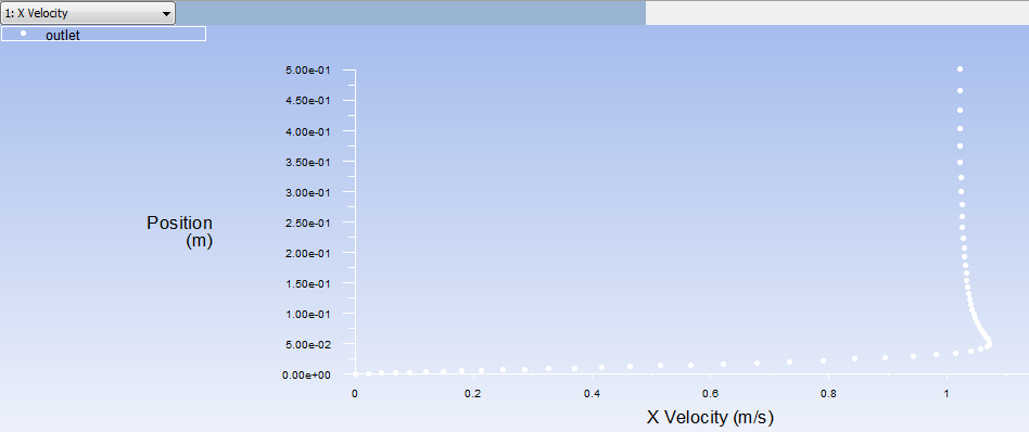
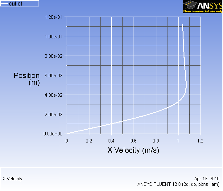
Now, click Plot. The plot of the x component of the velocity as a function of distance along the outlet now appears.




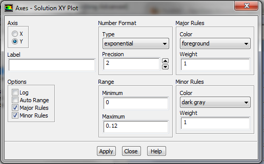
Now, the range of the y axis will be truncated, as we are not interested in far field velocity. Furthermore, the grid lines will be turned on. In order to implement these two changes. First click Axes in the Solution XY Plot menu. Next, select Y for Axis, deselect Auto Range, select Major Rules, select Minor Rules. Then, set Minimum to 0 and set Maximum to 1.2. Your Axes - Solution XY Plot menu, should look exactly like the image below.




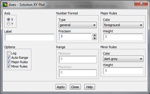
Then, click Apply in the Axes - Solution XY Plot menu. Now, select X for Axis and select Major Rules and Minor Rules, as shown below.




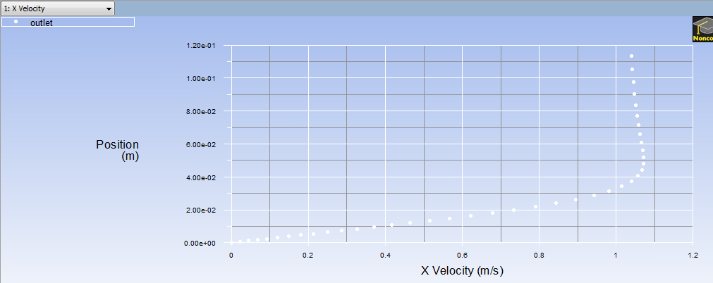
Next, click Apply in the Axes - Solution XY Plot menu. Close the Axes - Solution XY Plot menu. Now, click Plot menu in the Solution XY Plot menu. You should obtain the following output.




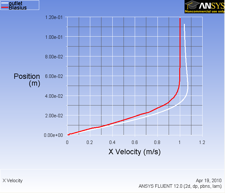
It is of interest to compare the numerical velocity profile to the velocity profile obtained from the Blasius solution. In order to plot the theoretical results, first click here to download the necessary file. Save the file to your working directory. Next, go to the Solution XY Plot menu and click Load File... and select the file that you just downloaded, _u_blasius_Re1e4.xy_. Lastly, click Plot in the Solution XY Plot menu. You should then obtain the following figure.

Plot Pressure Coefficients

Now we will display the pressure coefficient contour but first we need to set the reference values for velocity. Go back to:

Problem Setup > Reference Values

And select inlet under Compute From. Then go back to:

Results > Graphics and Animations > Graphics > Contours

Select Pressure...under Contours Of. Then select Pressure Coefficient from the second drop-down menu. Also, check the Filled checkbox and set Levels to 90. Then click on Display to update the display window.

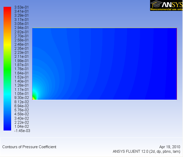
Zoom in at the leading edge.

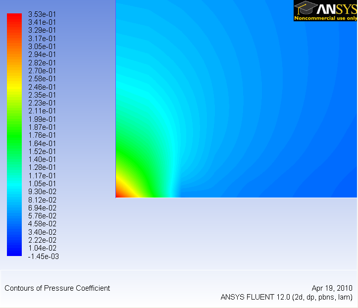
Why is the pressure not constant at the leading edge of the plate?

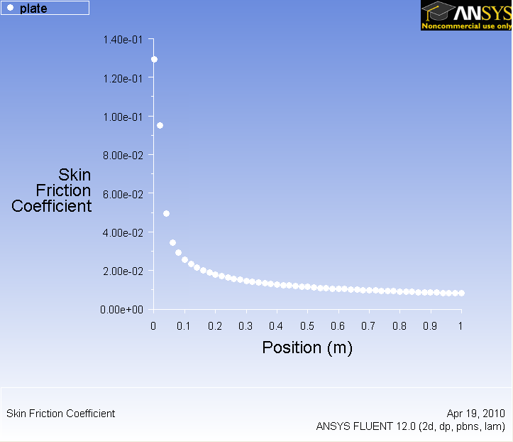
Plot Skin Friction Coefficient

Now we will plot the skin friction coefficient along the flat plate.

Results > Plots > XY Plot

Change Pressure to Wall Fluxes. Then, change Wall Shear Stress to Skin Friction Coefficient. Under Surfaces, select plate. 

 
Click Plot.
 

 

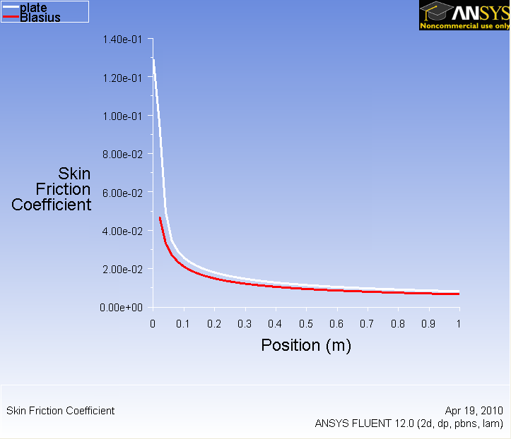
Now, compare your solution to the with the Blasius solution's skin friction by loading the file and then plotting it with your solution. (Download file here)

Also, you can change the symbol into lines by going to Curves... and click on the corresponding pattern that you like. Increase the Weight to 3 for readability. Both results should be fairly similar.

Plot Velocity Profiles

Results > Plots > XY Plot

Uncheck Position on X Axis and check Position on Y Axis under Options. Under Plot Direction, set X to 0 and Y to 1. Under X Axis Function, select Velocity...Then, change Velocity Magnitude to X Velocity. Finally under surface, select outlet. Before we are ready to plot, click on the Axes... button and rescale the y-axis from 0 to 0.12. Also, check the Major Rules and Minor Rules for both axes. Remember that you must click the Apply button when performing changes in each axis.

Click Plot.

To compare with the Blasius solution, download the solution here. Click Load File...and select the file you just downloaded. Then plot the solutions again to display both lines on the same graph.

What is the noticeably different between two solutions? Why is the velocity overshoot 1 for FLUENT's solution?

Now we will compare the velocity profile at two sections. Create another section in the middle of the plate.

Again, in the XY Plot window under New Surface > Line/Rake

Check the line tool checkbox under Options and set the initial coordinate to (0.5,0) and final coordinate to (0.5,0.5). Under the New Surface Name field, type in x_0.5 and then click the Create button to create the line.

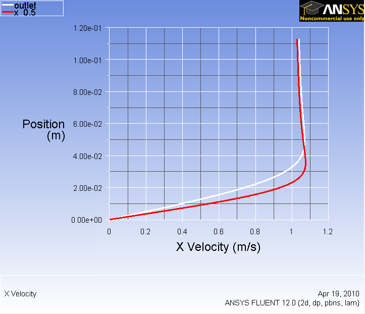
We can now plot and compare the velocity profile at the mid point and the outlet of the flow.

Under Surfaces, select outlet and {}x_0.5 and Plot.

Go to Step 7: Refine Mesh