FLUENT - Forced Convection - Step 4

Step 4: Setup (Physics)

In the Workbench window, this is what you should see currently in the Project Schematic space.

Double click on Setup which will bring up the FLUENT Launcher. Click OK to select the default options in the FLUENT Launcher. Twiddle your thumbs a bit while the FLUENT interface comes up. This is where we'll specify the governing equations and boundary conditions for our boundary-value problem. In the left-hand side of the FLUENT interface, we see various items listed under Problem Setup. We will work from top to bottom of the Problem Setup items to setup the physics of our problem. On the right hand side, we have the Graphics pane and, below that, the Command pane.

Display Mesh

 Let's first display the mesh that was created in the previous step. 

Problem Setup > General > Mesh > Display...

 
The long, skinny rectangle displayed in the graphics window corresponds to our solution domain. Some of the operations available in the graphics window to interrogate the geometry and mesh are:

Translation: The model can be translated in any direction by holding down the Left Mouse Button and then moving the mouse in the desired direction.

Zoom In: Hold down the Middle Mouse Button and drag a box from the Upper Left Hand Corner to the Lower Right Hand Corner over the area you want to zoom in on.

Zoom Out: Hold down the Middle Mouse Button and drag a box anywhere from the Lower Right Hand Corner to the Upper Left Hand Corner.

Use these operations to zoom in and interrogate our mesh.

You should have all the surfaces shown here.  You should check whether each surfaces correspond to the right geometry by unchecking unrelated surfaces and click Display to view the surface of interest in the Graphics window.

Next, we will specify that the problem we are solving is axisymmetric.
General > Solver > 2D Space > Axisymmetric

 
Now let's move on to setting up our model. We will first turn on the energy equation.
Models > Energy - Off > Edit...
Turn on the Energy Equation and click OK.
 
Next, we will setup the Viscous model.

Models > Viscous - Laminar > Edit...
Under Model, select k-epsilon (2 eqn) and click OK.

 
This is what you should currently see under Models.

 
Now let's move on to setting up the materials properties.
Materials > Fluid air >  Create/Edit...
We will use the properties of heated air. Change the Density (kg/m3) from constant to incompressible-ideal-gas.
Enter for following properties for air.
Cp (Specific Heat) (j/kg-k): 1005
Thermal Conductivity (w/m-k): 0.0266
Viscosity (kg/m-s): 1.787e-5
Molecular Weight (kg/kgmol): 28.97
 

Higher Resolution Image

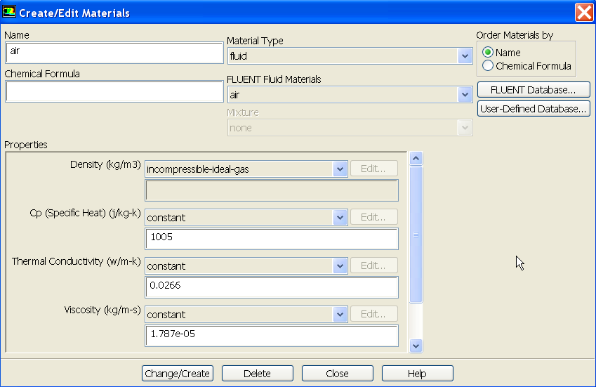
Click Change/Create and Close the Create/Edit Materials window.

Let's set up the boundary conditions now. We will first specify our operating conditions.

Boundary Conditions > Operating Conditions...

Enter 98338.2 under Operating Pressure and click OK.

Next we will specify boundary for centerline.

Boundary Conditions > centerline

Change the Type to  axis and click OK.

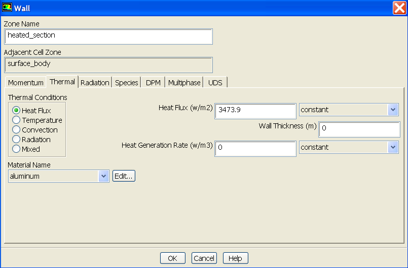
Now let's set up the heated wall section.

Boundary Conditions > heated_section > Edit...

A new Wall window will open. Click on Thermal tab and enter 3473.9 next to Heat Flux (w/m2) and click OK.

Higher Resolution Image

 
Now let's set the inlet boundary condition.
Boundary Conditions > inlet
Note that the boundary Type is automatically set to velocity-inlet. FLUENT has automatic mechanism to set the boundary condition according to the name you give. So let's click Edit... to set up the correct inlet parameters. A Velocity Inlet window pop out. Enter 25.05 next to Velocity Magnitude (m/s). For Turbulent Kinetic Energy (m2/s2), enter value 0.09. For Turbulent Dissipation Rate (m2/s3), enter value 16. Note that k and epsilon are not measured and are rough guess values. Click OK to close the window.

Higher Resolution Image

 
Now click on Thermal tab and enter 298.15K for Temperature. Click OK to close the window.
 
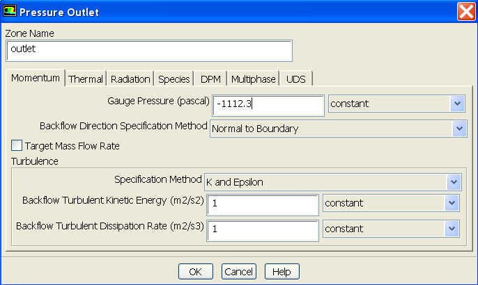
Finally, set up the outlet boundary condition.

Boundary Conditions > Outlet
Again, proper pressure-outlet boundary Type is set.  Click Edit... to set up appropriate pressure outlet condition. Enter -1112.3 for Gauge Pressure (From experiment, measured outlet pressure is 97225.9 Pa. Corresponding gauge pressure = 97225.9 Pa - reference pressure = -1112.3 Pa)

Higher Resolution Image

 
We are done setting up the boundary conditions.

Go to Step 5: Solution

See and rate the complete Learning Module

Go to all FLUENT Learning Modules