 Sign-up for free online course on ANSYS simulations!
Unable to render {include} The included page could not be found.
Step 1: Pre-Analysis
With the current problem setup, we know that the temperature will increase as the air passing through the heated section. Depending on whether the pipe is long enough, we might see uniform temperature at the end of the pipe.
Since the pipe cross-section is circular, we'll assume that the flow is axisymmetric. In cylindrical polar coordinates, this means that the flow variables depend only on the axial coordinate x and radial coordinate r, and are independent of the azimuthal coordinate θ. Hence we can model the pipe problem with a rectangular domain.
Figure above shows the simplified geometry of our problem where R = radius of the pipe, and L = length of the pipe.
ANSYS Simulation Flow
We are using FLUENT in solving this problem. With the new release of ANSYS 12, there have been a lot of improvement in term of overall flow. We start our simulation by first starting the ANSYS workbench.
Start > All Programs > ANSYS 12.0 > Workbench
Following figure shows the workbench window.

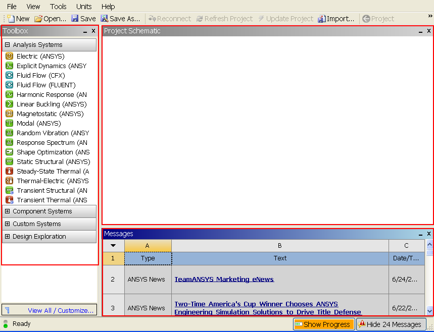
At the left hand side of the workbench window, you will see a toolbox full of various analysis systems. In the middle, you see an empty work space. This is the place where you will organize your project. At the bottom of the window, you see messages from ANSYS.
Since our problem involves fluid flow, we will select the FLUENT component on the left panel.
Left click (and hold) on Fluid Flow (FLUENT), and drag the icon to the empty space in the Project Schematic. Here's what you get:
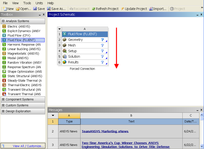
Since we selected Fluid Flow (FLUENT), each cell of the system corresponds to a step in the process of performing the FLUENT analysis. Rename the project to Forced Convection.
Now, we just need to work out each step from top down to get to the results for our solution.
- We start by preparing our geometry
- We use geometry to generate a mesh
- We setup the physics of the problem
- We run the problem in the solver to generate a solution
- Finally, we post process the solution to gain insight into the results