 Sign-up for free online course on ANSYS simulations!
Unable to render {include} The included page could not be found.
Author: John Singleton, Cornell University
Problem Specification
1. Pre-Analysis & Start-Up
2. Geometry
3. Mesh
4. Setup (Physics)
5. Solution
6. Results
7. Verification and Validation
Exercises
5. Solution
Download the solution by right-clicking the following link: conduction_2d.zip
Before we get ANSYS Mechanical to solve our boundary value problem, we have to tell it what results we would like to look at. In the solve step, ANSYS will obtain the temperature distribution in each element and from that populate the result items requested.
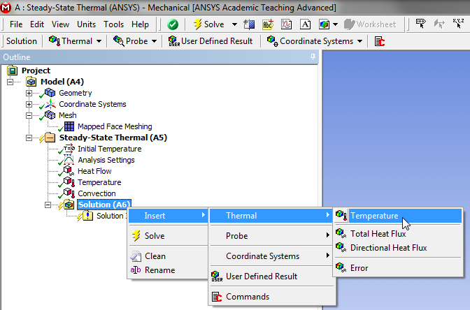
Temperature
To obtain the temperature distribution in the domain, (Right Click) Solution > Insert > Thermal > Temperature, as shown below.

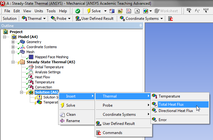
Total Heat Flux
To obtain the distribution of the total heat flux magnitude in the domain, (Right Click) Solution > Insert > Thermal > Total Heat Flux, as shown below.
x-Directional Heat Flux
To obtain the distribution of the x-directional heat flux in the domain, (Right Click) Solution > Insert > Thermal > Directional Heat Flux, as shown below.

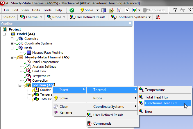
The default direction is set to x which suits us.This can be changed if necessary under the "Details of Directional Heat Flux" table.
Obtain the Numerical Solution
(Click) Solve,  . ANSYS will:
- obtain the element matrices
- assemble them into the global stiffness matrix
- invert the global stiffness matrix to obtain the temperature at the nodes
- populate the results requested from the nodal temperatures
Save
Save the project now. Do not close Mechanical.
Go to Step 6: Results
See and rate the complete Learning Module
Go to all ANSYS Learning Modules