 Sign-up for free online course on ANSYS simulations!
Step 6: Analyze Results
Lift Coefficient
The solution converged after about 480 iterations.
| No Format |
|---|
476 1.0131e-06 4.3049e-09 1.5504e |
| Wiki Markup |
{panel} [Problem Specification|FLUENT - Flow over an Airfoil- Problem Specification] [1. Create Geometry in GAMBIT|FLUENT - Flow over an Airfoil- Step 1] [2. Mesh Geometry in GAMBIT|FLUENT - Flow over an Airfoil- Step 2] [3. Specify Boundary Types in GAMBIT|FLUENT - Flow over an Airfoil- Step 3] [4. Set Up Problem in FLUENT|FLUENT - Flow over an Airfoil- Step 4] [5. Solve\!|FLUENT - Flow over an Airfoil- Step 5] {color:#ff0000}{*}6. Analyze Results{*}{color} [7. Refine Mesh|FLUENT - Flow over an Airfoil- Step 7] [Problem 1|FLUENT - Flow over an Airfoil- Problem 1] [Problem 2|FLUENT - Flow over an Airfoil- Problem 2] {panel} h2. Step 6: Analyze Results h4. Lift Coefficient The solution converged after about 1300 iterations. {noformat} iter continuity x-velocity y-velocity cl cd time/iter ! 1314 solution is converged 1314 9.7396e-07 4.7238e-09 1.7800e-09 6.4674e-01 2.4910e4911e-03 03 0:00:00 1 1315 1.0325e-06 4.6788e48 524 ! 477 solution is converged 477 9.9334e-07 4.2226e-09 1.7383e5039e-09 6.4675e4674e-01 2.4910e-03 03 0:00:00 38 0 {noformat} From FLUENT main window, we see that the lift coefficient is 523 |
From FLUENT main window, we see that the lift coefficient is 0.647.
...
This
...
compare
...
fairly
...
well
...
with
...
the
...
literature
...
result
...
of
...
0.6
...
from
...
...
...
al.
...
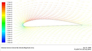
Plot Velocity Vectors
Let's
...
see
...
the
...
velocity
...
vectors
...
along
...
the
...
airfoil.
...
Display
...
>
...
Vectors
...
Enter
...
4
...
next
...
to
...
Scale
...
.
...
Enter
...
3
...
next
...
to
...
Skip
...
.
...
Click
...
Display.
| newwindow | ||||
|---|---|---|---|---|
| ||||
{_}{*}{color}. \\ !velocity magnitude_sm.jpg! {newwindow: Higher Resolution Image}https://confluence.cornell.edu/download/attachments/90744040/velocity%20magnitude.jpg{newwindow} \\ As can be |
As can be seen,
...
the
...
velocity
...
of
...
the
...
upper
...
surface
...
is
...
faster
...
than
...
the
...
velocity
...
on
...
the
...
lower
...
surface.
| Tip | ||||||||||||
|---|---|---|---|---|---|---|---|---|---|---|---|---|
| =
|
|
|
|
| |||||||
| } To get white background go to: *
Menu > File > Hardcopy *
sure that {color:#660099}{*}{_}Reverse Foreground/Background {_}{*}{color}is checked and select {color:#660099}{*}{_}Color {_}{*}{color}in {color:#660099}{*}{_}Coloring {_}{*}{color}section. Click {color:#660099}{*}{_}Preview {_}{*}{color}. Click {color:#660099}{*}{_}No {_}{*}{color}when prompted " _Reset graphics window?" |
| newwindow | ||||
|---|---|---|---|---|
| ||||
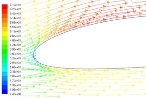
_" {tip} \\ \\ !velocity magnitude leading edge_sm.jpg! {newwindow: Higher Resolution Image} https://confluence.cornell.edu/download/attachments/90744040/velocity%20magnitude%20leading%20edge.jpg{newwindow} \\ On the leading |
On the leading edge,
...
we
...
see
...
a
...
stagnation
...
point
...
where
...
the
...
velocity
...
of
...
the
...
flow
...
is
...
nearly
...
zero.
...
The
...
fluid
...
accelerates
...
on
...
the
...
upper
...
surface
...
as
...
can
...
be
...
seen
...
from
...
the
...
change
...
in
...
colors
...
of
...
the vectors.
| newwindow | ||||
|---|---|---|---|---|
| ||||
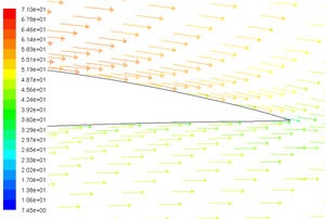
vectors. \\ !velocity magnitude trailing edge_sm.jpg! {newwindow: Higher Resolution Image}https://confluence.cornell.edu/download/attachments/90744040/velocity%20magnitude%20trailing%20edge.jpg{newwindow} \\ On the trailing |
On the trailing edge,
...
the
...
flow
...
on
...
the
...
upper
...
surface
...
decelerates
...
and
...
converge
...
with
...
the
...
flow
...
on
...
the
...
lower
...
surface.
| Info | ||
|---|---|---|
| ||
Do note that the time for fluid to travel top and bottom surface of the airfoil is not necessarily the same, as common misconception |
Plot Pressure Coefficient
Pressure Coefficient is a dimensionless parameter defined by the equation
| Latex |
|---|
where p is the static pressure,
Pref is the reference pressure, and
qref is the reference dynamic pressure defined by
| Latex |
|---|
The reference pressure, density, and velocity are defined in the Reference Values panel in Step 5. Please refer to FLUENT's help for more information. Go to Help > User's Guide Index for help.
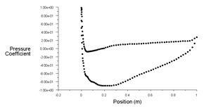
Plot > XY Plot...
Change the Y Axis Function to Pressure..., followed by Pressure Coefficient. Then, select airfoil under Surfaces.
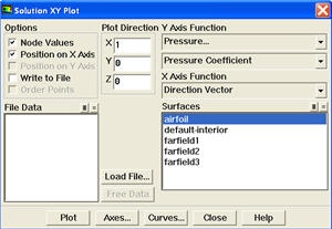
Click Plot.
| newwindow | ||||
|---|---|---|---|---|
| ||||
\\ {info:title=}Do note that the time for fluid to travel top and bottom surface of the airfoil is not necessarily the same, as common misconception {info} h4. Plot Pressure Coefficient *Pressure Coefficient* is a dimensionless parameter defined by the equation {latex} \large $$ {C_p} = {{(p-p_{ref})} \over q_{ref}} $$ {latex} where _p_ is the static pressure, _P{_}{_}{~}ref{~}_ is the reference pressure, and _q{_}{_}{~}ref{~}_ is the reference dynamic pressure defined by {latex} \large $$ q_{ref} = {1 \over 2}\rho_{ref}{v_{ref}}^2 $$ {latex} The reference pressure, density, and velocity are defined in the *Reference Values* panel in [Step 5|FLUENT - Flow over an Airfoil- Step 5]. Please refer to FLUENT's help for more information. Go to {color:#660099}{*}{_}Help > User's Guide Index{_}{*}{color} for help. *Plot > XY Plot...* Change the {color:#660099}{*}{_}Y Axis Function{_}{*}{color} to {color:#660099}{*}{_}Pressure{_}{*}{color}{color:#660099}...{color}, followed by {color:#660099}{*}{_}Pressure Coefficient{_}{*}{color}. Then, select {color:#660099}{*}{_}airfoil{_}{*}{color} under {color:#660099}{*}{_}Surfaces{_}{*}{color}. !pressure coefficient menu.jpg! Click {color:#660099}{*}{_}Plot{_}{*}{color}. \\ !pressure coefficient plot_sm.jpg!\\ {newwindow:Higher Resolution Image}https://confluence.cornell.edu/download/attachments/90744040/pressure%20coefficient%20plot.jpg{newwindow} |
The
...
lower
...
curve
...
is
...
the
...
upper
...
surface
...
of
...
the
...
airfoil
...
and
...
have
...
a
...
negative
...
pressure
...
coefficient
...
as
...
the
...
pressure
...
is
...
lower
...
than
...
the
...
reference
...
pressure.
...
Plot Pressure Contours
Plot static pressure contours.
Display > Contours...
...
Select Pressure...
...
and
...
Pressure
...
Coefficient
...
from
...
under
...
Contours
...
Of
...
.
...
Check
...
the
...
Filled
...
and
...
Draw
...
Grid
...
under
...
Options
...
menu.
...
Set
...
Levels
...
to
...
50.
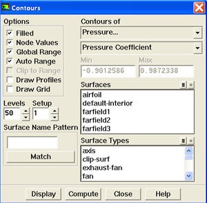
Click Display.
| newwindow | ||||
|---|---|---|---|---|
| ||||
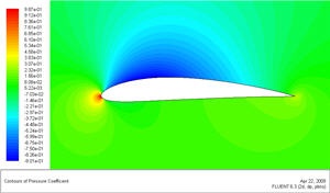
}}. \\ !presssure coefficient contour menu.jpg! Click {color:#660099}{*}{_}Display{_}{*}{color}. \\ \\ \\ !presssure coefficient contour plot_sm.jpg!\\ \\ {newwindow:Higher Resolution Image}https://confluence.cornell.edu/download/attachments/90744040/presssure%20coefficient%20contour%20plot.jpg{newwindow} From the contour of pressure coefficient, we see that there is a region of high pressure at the leading edge (stagnation point) and region of low pressure on the upper surface of airfoil. This is of what we expected from analysis of velocity vector plot. From Bernoulli equation, we know that whenever there is high velocity, we have low pressure and vise versa. Before we can make any conclusion about the accuracy of our result, we should always make validation check. The most common validation step is grid convergence check. h4. Comparisons With our simulation data, we can now compare the Fluent with experimental data. The summary of result is shown in the table. | \\ | CL | Cd | | FLUENT | 0.647 \\ | 0.00249 \\ | | Experiment | 0.6 \\ | 0.007 | | Theory | \- | 0 | {info:title= }The experimental data is taken from *Theory of Wing Sections* By Ira Herbert Abbott, Albert Edward Von Doenhoff pg. 493 {newwindow: Google scholar link}http://books.google.com/books?id=DPZYUGNyuboC&printsec=frontcover&dq=Theory+of+Wing+Sections&ei=u6a6SZLfBJ6cMtj-iOcL#PPA489,M1{newwindow} {info} \\ Go to [Step 7: Refine Mesh|FLUENT - Flow over an Airfoil- Step 7] [See and rate the complete Learning Module|FLUENT - Flow over an Airfoil] Go to [all FLUENT Learning Modules|FLUENT Learning Modules] |
From the contour of pressure coefficient, we see that there is a region of high pressure at the leading edge (stagnation point) and region of low pressure on the upper surface of airfoil. This is of what we expected from analysis of velocity vector plot. From Bernoulli equation, we know that whenever there is high velocity, we have low pressure and vise versa.
Go to Step 7: Refine Mesh