 Sign-up for free online course on ANSYS simulations!
| Panel |
|---|
Author: Rajesh Bhaskaran & Yong Sheng Khoo, Cornell University Problem Specification |
Step 6:
...
Results
| Info | ||
|---|---|---|
| ||
These instructions are for FLUENT 6.3.26. Click here for instructions for FLUENT 12. |
Velocity Vector
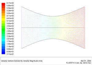
Let's first look at the velocity vector in the nozzle.
Display > Vectors...
Select Velocity under Vectors of and Velocity... under Color by. Set Scale to 0.4
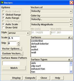
Click Display.
| newwindow | ||||
|---|---|---|---|---|
| ||||
https://confluence.cornell.edu/download/attachments/90741106/velocity-vector-result.jpg?version=1 |
We see that the flow is smoothly accelerating from subsonic to supersonic.
| Info | ||
|---|---|---|
| ||
Display > Views... |
| Info | ||
|---|---|---|
| ||
To get white background go to: |
...
Mach Number Contour
Let's now look at the mach Mach number
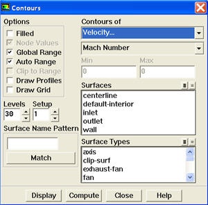
Display > Contours
Select Velocity... under Contours of and select Mach Number. Set Levels to 30.
| newwindow | ||||
|---|---|---|---|---|
| ||||
https://confluence. |
...
cornell.edu/download/attachments/90741106/mach-contour-result.jpg?version=1 |
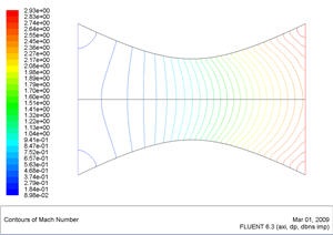
For 1D case, mach number is a function of x position. For 1D case, we are supposed to see vertical contour of mach numbers that are parallel to each other.
For 2D case, we are seeing curving contour of mach number. The deviation from vertical indicates the 2D effect.
Do note that 1D approximation is fairly accurate around the centerline of nozzle.
Pressure Contour Plot
Let's look at how pressure changes in the nozzle.
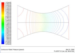
Display > Contours...
Select Pressure... and Static Pressure under Contours of. Use Levels of 30
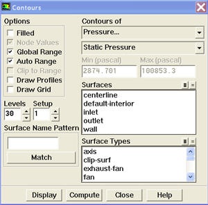
Click Display.
| newwindow | ||||
|---|---|---|---|---|
| ||||
https://confluence.cornell.edu/download/attachments/90741106/pressure-contour-result.jpg?version=1 |
Notice that the pressure decreases as it flows to the right.
Total Pressure Contour Plot
Let's look at the total pressure in the nozzle
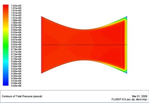
Display > Contours...
Select Pressure... and Total Pressure under Contours of. Select Filled. Use Levels of 100.
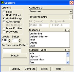
Click Display.
| newwindow | ||||
|---|---|---|---|---|
| ||||
https://confluence.cornell.edu/download/attachments/90741106/totalpressure-contour-result.jpg?version=1 |
Around the nozzle outlet, we see that there is a pressure loss because of the numerical dissipation.
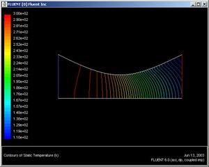
Temperature Contour Plot
Let's investigate or verify the temperature properties in the nozzle
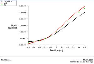
Mach Number Plot
As in the previous tutorials, we are going to plot the velocity along the centerline. However, this time, we are going to use the dimensionless Mach quantity.
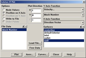
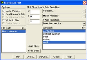
Plot > XY Plot
We are going plot the variation of the Mach number in the axial direction at the axis and wall. In addition, we will plot the corresponding variation from 1D theory. You can download the file here: mach_1D.xy.
Do everything as we would do for plotting the centerline velocity. However, instead of selecting Axial Velocity as the Y Axis Function, select Mach Number.
Also, since we are going to plot this number at both the wall and axis, select centerline and wall under Surfaces.
Then, load the mach_1D.xy by clicking on Load File....
(Click picture for large image)
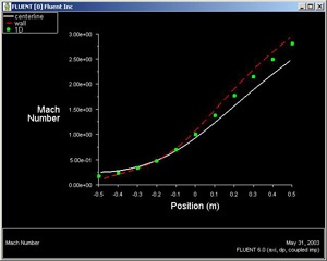
Click Plot.
(Click picture for large image)
How does the FLUENT solution compare with the 1D solution?
Is the comparison better at the wall or at the axis? Can you explain this?
Save this plot as machplot.xy by checking Write to File and clicking Write....
Pressure Contour Plot
Sometimes, it is very useful to see how the pressure and temperature changes throughout the object. This can be done via contour plots.
Display > Contours...
First, we are going to plot the pressure contours of the nozzle. Therefore, make sure that under Contours Of, Pressure... and Static Pressure is selected.
We want this at a fine enough granularity so that we can see the pressure changes clearly. Under Levels, change the default 20 to 40. This increases the number of lines in the contour plot so that we can get a more accurate result.
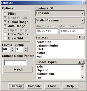
Click Display.
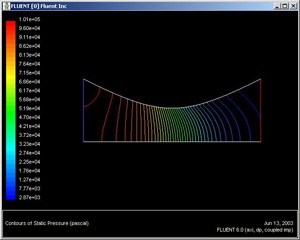
(Click picture for large image)
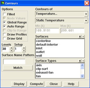
Select Temperature... and Static Temperature under Contours of. Use Levels of 30.

| newwindow | ||||
|---|---|---|---|---|
| ||||
https://confluence.cornell.edu/download/attachments/90741106/temperature-contour-result.jpg?version=1 |
As we can see, the temperature decreases from left to right in the nozzle, indicating a transfer of internal energy to kinetic energy as the fluid speeds up.
Total Temperature Contour Plot
Let's look at the total pressure in the nozzle
Display > Contours...
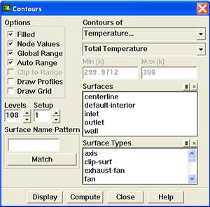
Select Temperature... and Total Temperature under Contours of. Select Filled. Use Levels of 100.
| newwindow | ||||
|---|---|---|---|---|
| ||||
https://confluence.cornell.edu/download/attachments/90741106/totaltemperature-contour-result.jpg?version=1 |
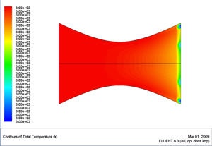
Looking at the scale, we see that the total temperature is uniform 300 K throughout the nozzle. The contour abnormality at the outlet of the nozzle is due to the round off errorsNotice that the pressure on the fluid gets smaller as it flows to the right, as is consistent with fluid going through a nozzle.
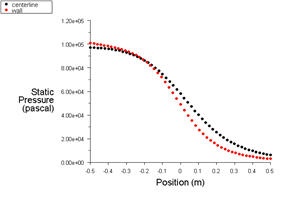
Pressure Plot
Let's look at the pressure along the centerline and the wall.
Plot > XY Plot
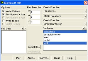
Make sure that under Y-Axis Function, you see Pressure... and Static Pressure. Under Surfaces, select centerline and wall. Click Plot.
| newwindow | ||||
|---|---|---|---|---|
| ||||
https://confluence.cornell.edu/download/attachments/90741106/pressure-plot-result.jpg?version=1 |
It is good to write the data into a file to have greater flexibility on how to present the result in the report. At the same XY Plot windows, select Write to File. Then click Write... Name the file "p.xy" in the directory that you prefer.
Open "p.xy" file with notepad or other word processing software. At the top, we see:
...
Try copy the appropriate data sets to excel and plot the results.
Temperature Contour Plot
Mach Number Plot
Let's plot the variation of Mach number in the axial direction at the axis and wall. In addition, Now we will plot the temperature contours and see how the temperature varies throughout the nozzle.
Back in the Contours window, under Contours Of, select Temperature... and Static Temperature.
Click Display.
(Click picture for large image)
corresponding variation from 1D theory. You can download the file here: mach_1D.xy.Plot > XY PlotUnder the Y Axis Function, select Velocity... and Mach Number.
Also, since we are going to plot this number at both the wall and axis, select centerline and wall under Surfaces.
Then, load the mach_1D.xy by clicking on Load File....
Click Plot.
| newwindow | ||||
|---|---|---|---|---|
| ||||
https://confluence.cornell.edu/download/attachments/90741106/mach-plot-result.jpg?version=1 |
How does the FLUENT solution compare with the 1D solution?
Is the comparison better at the wall or at the axis? Can you explain this?
Save this plot as machplot.xy by checking Write to File and clicking Write...As we can see, the temperature decreases towards the right side of the nozzle, indicating a change of internal energy to kinetic energy as the fluid speeds up.
Go to Step 7: Refine MeshVerification & Validation