 Sign-up for free online course on ANSYS simulations!
| Include Page | ||||
|---|---|---|---|---|
|
| Include Page | ||||
|---|---|---|---|---|
|
Pre-Analysis and Start-Up
Pre-Analysis
...
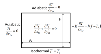
The figure below illustrates the given non-dimensional boundary value problem.

| newwindow | ||||
|---|---|---|---|---|
|
https://confluence.cornell.edu/download/attachments/146918509/ProbPic_Full.png |
...
ANSYS solves the dimensional form of the boundary value problem as shown below.
| newwindow | ||||
|---|---|---|---|---|
| ||||
https://confluence.cornell.edu/download/attachments/146918509/DimForm_Full.png |
...
Here
| Wiki Markup |
|---|
{latex} $x_D$ {latex} |
...
| Wiki Markup |
|---|
{latex} $y_D$ {latex} |
...
...
the
...
dimensional
...
coordinates.
...
We
...
will
...
choose
...
the
...
dimensions
...
and
...
boundary
...
condition
...
inputs
...
such
...
that
...
the
...
dimensional
...
problem
...
matches
...
the
...
non-dimensional
...
one.
...
Then,
...
T
...
values
...
in
...
Celsius
...
that
...
ANSYS
...
reports
...
can
...
be
...
interpreted
...
as
| Wiki Markup |
|---|
{latex} $\theta$ {latex} |
...
For
...
the
...
geometry,
...
we pick
| Wiki Markup |
|---|
pick {latex} \[ W = 1m, \ \ H = 2 m \] {latex} |
For
...
the
...
boundary
...
conditions,
...
we pick
| Wiki Markup |
|---|
pick {latex} \[ T_0 = 1, \ \ k = 1, \ \ T_\infty=0 \ \ h = Bi \] {latex} |
These
...
are
...
the
...
inputs
...
we'll
...
use
...
while
...
setting
...
up
...
the
...
problem
...
in
...
ANSYS.
...
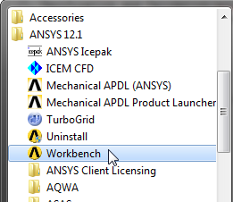
Open
...
ANSYS
...
Workbench
Launch ANSYS Workbench from the Start menu as shown below.
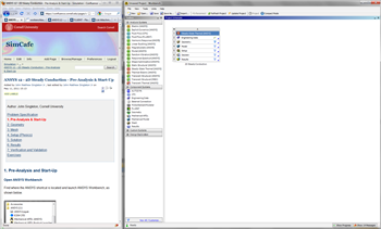
Management of Screen Real Estate
This tutorial is specially configured so that the user can have both the tutorial and ANSYS open at the same time as shown below. It will be beneficial to have both ANSYS and your internet browser displayed on your monitor simultaneously. Your internet browser should consume approximately one third of the screen width while ANSYS should take the other two thirds as shown below.
| newwindow | ||||
|---|---|---|---|---|
| ||||
https://confluence.cornell.edu/download/attachments/146918509/RealEstate_Full.png |
...
If the monitor you are using is insufficient in size, you can press the Alt and Tab keys simultaneously to toggle between ANSYS and your internet browser.
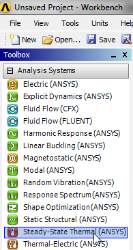
Steady-State Thermal Analysis System
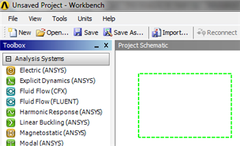
The problem at hand is a steady state thermal problem, thus the steady-state thermal analysis system will be used. Click on Steady-State Thermal(ANSYS) as shown in the image below.
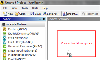
Continue to hold down the left mouse button and drag Steady-State Thermal(ANSYS) into the Project Schematic area. You will then see a green rectangle appear as shown below.
Drag Steady-State Thermal(ANSYS) to the green box which will then turn red and contain text saying "Create standalone system".
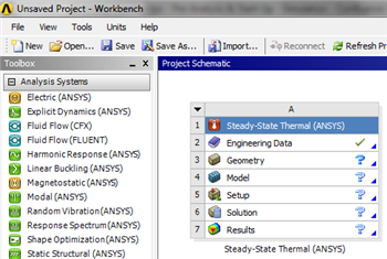
Now, release the left mouse button to create the standalone system. Your Project Schematic window should look comparable to the image below.
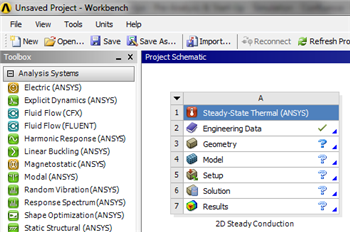
Lastly, rename the system to "2D Steady Conduction", as shown below.
Engineering Data
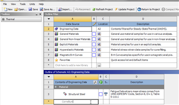
In this section the material properties that appear in the boundary value problem will be specified. In our case, the only material property that appears in the boundary value problem is k, the coefficient of thermal conductivity. ANSYS requires a name for the material, so we'll call it "Cornellium". First (Double Click) Engineering Data. Then click in the cell that contains the text "Click here to add a new material" and type in Cornellium as shown below.
| newwindow | ||||
|---|---|---|---|---|
| ||||
https://confluence.cornell.edu/download/attachments/146918509/EngData1_Full.png |
...
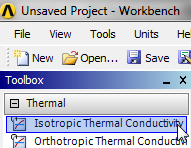
Next, (Expand)
...
Thermal
...
and
...
(Double
...
Click)
...
Isotropic
...
Thermal
...
Conductivity
...
,
...
as
...
shown
...
below.
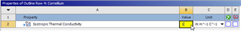
Then, set the value of the Isotropic Thermal Conductivity to 1 W/(M*C)
...
as
...
shown
...
below.
| newwindow | ||||
|---|---|---|---|---|
| ||||
https://confluence.cornell.edu/download/attachments/146918509/EngData3_Full.png |
...
Lastly,
...
click
...
Return
...
to
...
Project
...
,  , in order to return to the Project Schematic window.
Saving
It would be in our best interest to save the project at this point. Click on the Save As.. button,  , which is located on the top of the Workbench window. Save the project as "SteadyConduction". When you save in ANSYS, a file and a folder will be created. For instance if you save as "SteadyConduction", a "SteadyConduction.wbpj" file and a folder called "SteadyConduction_files" will appear. In order to reopen the ANSYS files in the future you will need both the ".wbpj" file and the folder. If you do not have BOTH, you will not be able to access your project.
Go to Step 2: Geometry
Go to all ANSYS Learning Modules