Sign-up for free online course on ANSYS simulations!
| Include Page | ||||
|---|---|---|---|---|
|
...
|
...
|
...
|
| Include Page | ||||
|---|---|---|---|---|
|
Numerical Results
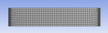
Before we explore the ANSYS results, let's take a peek at the mesh.
Mesh
Click on Mesh (above Solution) in the tree outline. This shows the mesh used to generate the ANSYS solution. The domain is a rectangle. This domain is discretized into a number of small "elements". Recall that ANSYS solves the BVP and calculates the displacements at the nodes. A finer mesh is used near the left and right ends where we expect greater stress concentration. We have checked that the solution presented to you is reasonably independent of the mesh.
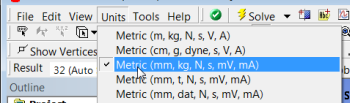
Units
Set the units for the results display by selecting Units > Metric (mm, kg, N, s, mV, mA). The displacements will be reported in mm and the stresses in N/mm2 which is equivalent to MPa.
Displacement
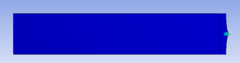
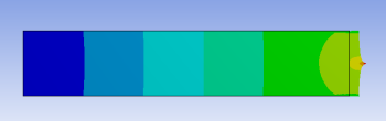
To view the deformed structure, click on Solution > Displacement in the tree outline. The black rectangle shows the undeformed structure. The deformed structure is colored by the magnitude of the displacement. The displayed displacement distribution is calculated by interpolating the nodal displacements. Red areas have deformed more and blue areas less. You can see that the left end has not moved as specified in the problem statement. This means this boundary condition has been applied correctly. The displacement increases from left to right as we intuitively expect. There is also not much variation in the y-direction. So we can conclude that the model has been constrained properly.
Note the extremely high deformation near the point load. This extremum is unrealistic and should be ignored (there are no point loads in reality).
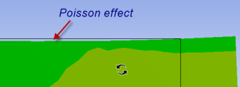
To view the Poisson effect (shrinking in the y direction), zoom into the top-rightright corner by drawing a rectangle around the region with the right mouse button.

You can do this multiple times to zoom in more. You do indeed see the shrinking in the y-direction as expected but it is small for this model.
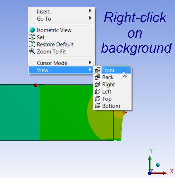
You can restore the front view of the entire model by right-clicking in the background and choosing View > Front.
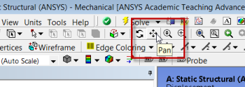
Note that you can zoom in and out using the middle mouse wheel. You can translate the model by clicking on the Pan button and dragging the model with the left mouse button. There are also a bunch of zoom options next to the Pan button.
sigma_x
The stresses are derived from the nodal displacements using Hooke's law. In the following video, we look at the sigma_x distribution in the interior and at the boundaries and compare the ANSYS values to the values expected from the analytical solution and traction boundary conditions.
| Wiki Markup |
|---|
} {include: ANSYS Google Analytics} h1. Numerical Results Before we explore the ANSYS results, let's take a peek at the mesh. h3. Mesh Click on {color:purple}{*}{_}Mesh{_}{*}{color} (above {color:purple}{*}{_}Solution{_}{*}{color}) in the tree outline. This shows the mesh used to generate the ANSYS solution. The domain is a rectangle. This domain is discretized into a number of small "elements". Recall that ANSYS solves the BVP and calculates the displacements at the nodes. A finer mesh is used near the left and right ends where we expect greater stress concentration. We have checked that the solution presented to you is reasonably independent of the mesh. \\ !mesh.png!\\ h3. Units Set the units for the results display by selecting {color:#990099}{*}{_}Units > Metric (mm, kg, N, s, mV, mA)_{*}{color}. The displacements will be reported in _mm_ and the stresses in _N/mm2_ which is equivalent to _MPa_. !units.png|border=1! h3. Displacement To view the deformed structure, click on {color:purple}{*}{_}Solution > Displacement{_}{*}{color} in the tree outline. The black rectangle shows the undeformed structure. The deformed structure is colored by the magnitude of the displacement. The displayed displacement distribution is calculated by interpolating the nodal displacements. Red areas have deformed more and blue areas less. You can see that the left end has not moved as specified in the problem statement. This means this boundary condition has been applied correctly. The displacement increases from left to right as we intuitively expect. There is also not much variation in the y-direction. So we can conclude that the model has been constrained properly. Note the extremely high deformation near the point load. This extremum is unrealistic and should be ignored (there are no point loads in reality). !tut1 displacement.png! To view the Poisson effect (shrinking in the y direction), zoom into the top-rightright corner by drawing a rectangle around the region with the _right_ mouse button. !zoom_corner.png|border=1! You can do this multiple times to zoom in more. You do indeed see the shrinking in the y-direction as expected but it is small for this model. !poisson_effect.png|border=1! You can restore the front view of the entire model by right-clicking in the background and choosing {color:purple}{*}{_}View > Front{_}{*}{color}. !front_view.png|border=1! Note that you can zoom in and out using the middle mouse wheel. You can translate the model by clicking on the _Pan_ button and dragging the model with the left mouse button. There are also a bunch of zoom options next to the _Pan_ button. !pan.png|border=1! h3. sigma_x The stresses are derived from the nodal displacements using Hooke's law. In the following video, we look at the sigma_x distribution in the interior and at the boundaries and compare the ANSYS values to the values expected from the analytical solution and traction boundary conditions. \\ {html}<iframe width="600" height="338" src="//www.youtube.com/embed/vBNFUYrsWMw?rel=0" frameborder="0" allowfullscreen></iframe>{html} \\ |
In
...
the
...
video,
...
we
...
saw
...
that
...
ANSYS's
...
values
...
for
...
sigma_x
...
matches
...
with:
...
- The
...
- analytical
...
- solution
...
- in
...
- the
...
- interior
...
- (away
...
- from
...
- the
...
- left
...
- and
...
- right
...
- boundaries)
...
- Traction
...
- boundary
...
- condition
...
- for
...
- sigma_x
...
- at
...
- the
...
- right
...
- boundary
...
Note
...
- that
...
- sigma_x
...
- at
...
- the
...
- location
...
- of
...
- the
...
- point
...
- load
...
- is
...
- infinite.
...
- So
...
- as
...
- the
...
- mesh
...
- is
...
- refined
...
- further,
...
- sigma_x
...
- at
...
- the
...
- point
...
- load
...
- will
...
- get
...
- larger
...
- and
...
- larger
...
- without
...
- bound.
...
sigma_y
...
Next,
...
let's
...
take
...
a
...
look
...
at
...
sigma_y.
...
Click
...
on
...
Solution
...
>
...
sigma_y
...
in
...
the
...
tree
...
outline.
...
Again,
...
probe
...
values
...
in
...
the
...
middle
...
as
...
well
...
as
...
at
...
the
...
ends.
...
Check
...
that:
...
- The
...
- value
...
- away
...
- from
...
- the
...
- boundaries
...
- is
...
- close
...
- to
...
- zero
...
- as
...
- expected
...
- from
...
- the
...
- analytical
...
- solution.
...
- It
...
- is
...
- not
...
- exactly
...
- zero
...
- because
...
- of
...
- round-off
...
- errors.
...
- The
...
- value
...
- at
...
- the
...
- top
...
- and
...
- bottom
...
- boundaries
...
- are
...
- close
...
- to
...
- zero.
...
- This
...
- agrees
...
- with
...
- the
...
- boundary
...
- condition
...
- at
...
- these
...
- boundaries
...
- since
...
- the
...
- traction
...
- has
...
- to
...
- be
...
- zero
...
- at
...
- these
...
- free
...
- boundaries.
...
- In
...
- other
...
- words,
...
- the
...
- normal
...
- component
...
- of
...
- the
...
- traction
...
- acting
...
- on
...
- these
...
- surfaces
...
- is
...
- sigma_y
...
- and
...
- that
...
- has
...
- to
...
- be
...
- zero
...
- since
...
- the
...
- traction
...
- on
...
- these
...
- free
...
- surfaces
...
- is
...
- zero.
...
- There
...
- is
...
- significant
...
- deviation
...
- from
...
- the
...
- analytical
...
- solution
...
- at
...
- both
...
- ends.
...
- The
...
- analytical
...
- solution
...
- breaks
...
- down
...
- at
...
- these
...
- ends
...
- because
...
- of
...
- the
...
- additional
...
- assumptions
...
- that
...
- we
...
- made.
...
- Note
...
- that
...
- there
...
- are
...
- areas
...
- where
...
- sigma_y
...
- is
...
- negative
...
- i.e.
...
- compressive.

tau_xy
...
We
...
expect
...
tau_xy
...
to
...
be
...
zero
...
away
...
from
...
the
...
ends.
...
Near
...
the
...
ends,
...
since
...
sigma_x
...
and
...
sigma_y
...
are
...
non-zero,
...
we expect
| Wiki Markup |
|---|
expect \\ {latex} \[ \tau_{xy} = \tau_{xy}(x,y) \] {latex} |
Plot
...
tau_xy,
...
look
...
at
...
the
...
range
...
of
...
values
...
and
...
use
...
Probe
...
to
...
check
...
actual
...
values.
...
Are
...
the
...
above
...
statements
...
valid?
Equivalent Stress (Von Mises):
The Equivalent or Von Mises stress is used to predict yielding of the material. We can see that the analytical solution under-predicts the maximum equivalent stress. Thus, one would need to use a large factor of safety if using the analytical result while designing such a structure. One would use a factor of safety with the FEA result also but it does not have to be as large.