...

Numerical Results

Displacement

Okay! Now let's look at the numerical solution to the boundary value problem as calculated by ANSYS. Let's start by examining how the plate deformed under the load. Before you start, make sure the software is working in the same units you are by looking to the menu bar and selecting Units > US Customary (in, lbm, lbf, F, s, V, A). Also, select the pan tool by clicking the pan button from the top bar. This will allow you to zoom by scrolling the mouse wheel, and move the image by left-clicking and dragging.

...

To get back the color contours of deformation values, select the Contours button and choose Contour Bands. The colored section refers to the magnitude of the deformation (in inches) while the black outline is the undeformed geometry superimposed over the deformed model. The more red a section is, the more it has deformed while the more blue a section is, the less it has deformed. Notice that far from the hole, the deformation is linearly varying, similar to a bar in tension. Now let's look at the value of the largest deformation. Looking at the top of the color bar, we see that the largest deformation is 0.17605 inches. From our pre-analysis, we found that the deformation was 0.1724 inches - a 2% difference. Being that our calculation was only an estimate (we neglected the hole), this seems reasonable.

Sigma-r

Now let's look at the radial stresses in the plate. Look to the outline window and click Solution > Sigma-r. This will display the radial stresses.

...

Now, let's first look at the case when r >> a. As we found in the pre-calculations, when r >> a, the radial stress is a function of the angle theta only. This matches the behavior seen in the simulation. From our Pre-Calculations, we also found that 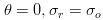. Using the probe tool, we find that indeed at this location, the stress is equal to 1e6 psi, which is the value we calculated in our Pre-Analysis. Also from our Pre-Analysis, we found that when .
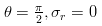Checking the simulation with our trusty probe tool, we find that the ANSYS simulation matches up quite nicely with our calculation.

Sigma-Theta

Now, let's compare the simulation to our pre-calculations for the theta stress. Look to the Outline window, then click Solution > Sigma-theta

...

Now, let's look at the case when r >> a. From our pre-calculations, we found that the theta stress is a function of theta only. This behavior is represented in the simulation. Also, for r >> a and the stress is equal to .
Using the probe tool and hovering over this area, we see that the stress is indeed equal to Sigma-o. However, looking at the area when , we find that the stress from the simulation is between 1000 psi and 2000 psi. Although this seems large compared to zero, one must keep in mind that the stress at this location is 1% of the average stress. We expect that the stress here will get closer to zero on refining the mesh since the numerical error becomes smaller.

Tau-r-theta

Now let's look at how the simulation match our predictions for the shear stress. Look to the Outline window, then click Solution > Tau-r-theta

...

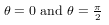
In our pre-calculations, we determined that far from the hole the shear stress should be a function of theta only. This can be shown by using the probe tool a hovering over a radial line from the hole. The colors (representing higher and lower stresses) only change only as the angle changes, but not as the move away from the hole. We also found that far from the hole at the stress is zero

Using the probe tool, we can see that this is indeed the case for the simulation as well.

Sigma-x

Now lets examine the stress in the x-direction. Look to the Outline window, then click Solution > Sigma-x

...