...
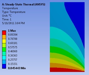
To view the Temperature over the surface, select Solution > Temperature from the tree on the left.
| newwindow |
|---|
| Click Here for Higher Resolution |
|---|
| Click Here for Higher Resolution |
|---|
|
https://confluence.cornell.edu/download/attachments/146918520/UnrefTemp_Full.PNG |
In order to view the Isolines of the object, select the viewing button, and change from Contour Bands into Isolines. 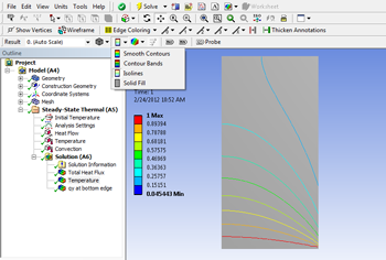 Image Added
| newwindow |
|---|
| Click Here for Higher Resolution |
|---|
| Click Here for Higher Resolution |
|---|
|
https://confluence.cornell.edu/download/attachments/146918520/Isolines.png |
Total Heat Flux
We would now like to view the Total Heat Flux as vectors, in order to better visualize it, as well as to check the perfectly insulated boundaries. In order to do so, select Solution > Total Heat Flux from the tree on the left. Then (Click) Vectors,  . The sliders in the top bar can be used to change the size and number of vectors displayed. At this point, the heat flux should appear similar to the image below.
...
| newwindow |
|---|
| Click Here for Higher Resolution |
|---|
| Click Here for Higher Resolution |
|---|
|
https://confluence.cornell.edu/download/attachments/146918520/DirHeatFluxVec_Full.png |
X Direction Heat Flux
...
https://confluence.cornell.edu/download/attachments/146918520/UnrefDirectHeatFluxXX_Full.PNG
Temperature along Y=1m line
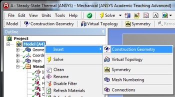
At this point we are interested in extracting the temperature values along the horizontal line, y=1m. This is done by defining a "path" and sampling the temperature along this path. First, (Right Click) Model > Insert > Construction Geometry as shown below.
| newwindow |
|---|
| Click Here for Higher Resolution |
|---|
| Click Here for Higher Resolution |
|---|
|
https://confluence.cornell.edu/download/attachments/146918520/InsConstructGeomFull.PNG |
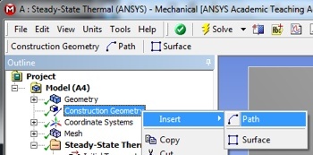
Next,
(Right Click) Construction Geometry > Insert > Path as shown in the following image.
| newwindow |
|---|
| Click Here for Higher Resolution |
|---|
| Click Here for Higher Resolution |
|---|
|
https://confluence.cornell.edu/download/attachments/146918520/InsertPath_Full.PNG |
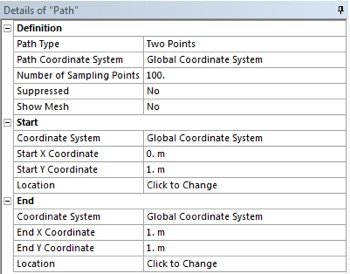
Then, set
Number of Sampling Points to 100, set
Start X Coordinate to 0, set
Start Y Coordinate to 1, set
End X Coordinate to 1, and set
End Y Coordinate to 1 as shown below.
| newwindow |
|---|
| Click Here for Higher Resolution |
|---|
| Click Here for Higher Resolution |
|---|
|
https://confluence.cornell.edu/download/attachments/146918520/PathDet_Full.PNG |
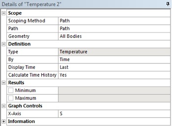
At this point another temperature output must be created. In order to create the temperature output
(Right Click) Solution > Insert > Thermal > Temperature. In the "Details of Temperature 2" table set the
Scoping Method to
Path as shown below. Then, set
Path to
Path. Your "Details of Temperature 2" table should now look like the following image.
| newwindow |
|---|
| Click Here for Higher Resolution |
|---|
| Click Here for Higher Resolution |
|---|
|
https://confluence.cornell.edu/download/attachments/146918520/DetTemp2_Full.PNG |
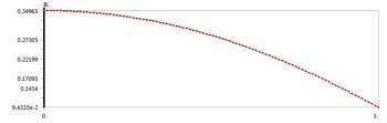
Now,
(Click) Solve,

, and ANSYS will find the temperature on the line y=1 m as a function of x position. ANSYS will obtain the temperature for 100 points on the line y=1m. The data points are displayed in a table and can be exported to MATLAB or EXCEL. The following image shows, the graph that ANSYS outputs. The y axis is non-dimensional temperature and the x axis is x position on the line y=1m.
| newwindow |
|---|
| Click Here for Higher Resolution |
|---|
| Click Here for Higher Resolution |
|---|
|
https://confluence.cornell.edu/download/attachments/146918520/PathTempResults_Full.PNG |
...
Now,(Click) Solve, , and ANSYS will find the Directional Heat Flux on the line y=0m as a function of x position. We would like to find the Total Heat Flux through the bottom, and to by integrating the flux along that boundary. To do this we will export the data to MATLAB and perform a numerical integration. To do so, right click in the tabular data displayed in the lower righthand corner of the screen. Select all (Ctrl+A), right-click and select Export. Save the file as "qy_bot.txt" in your MATLAB working directory.
...
 Sign-up for free online course on ANSYS simulations!