 Sign-up for free online course on ANSYS simulations!
| Include Page |
|---|
...
|
...
|
| Include Page |
|---|
...
|
...
|
Numerical Results
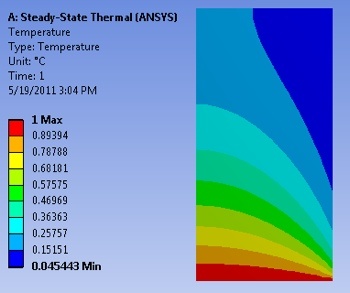
Temperature
To view the temperature distribution over the surface, select Solution > Temperature from the tree on the left.
...
https://confluence.cornell.edu/download/attachments/146918520/UnrefTemp_Full.PNG
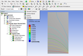
Temperature Contours
In order to view the contours as isolines, select the viewing button, and change from Contour Bands into Isolines.
...
https://confluence.cornell.edu/download/attachments/146918520/Isolines.pngTotal Heat Flux
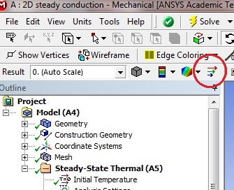
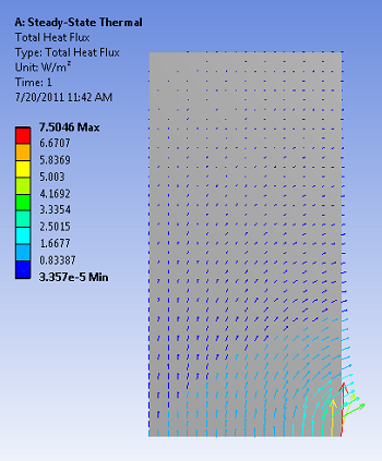
We will view the heat flux as vectors. This will tell us the direction of heat flow within the geometry as well as at the boundaries In order to plot the heat flux vectors, select Solution > Total Heat Flux from the tree on the left. Then (Click) Vectors,  near the top of the GUI. The sliders in the top bar can be used to change the size and number of vectors displayed.
...
At this point, the heat flux vectors should appear similar to the image below. Take a minute to think about whether the heat flow directions at the boundaries match what you expect.
...
https://confluence.cornell.edu/download/attachments/146918520/DirHeatFluxVec_Full.pngHeat Flux Variation Along Bottom Surface
We'll plot the heat flux crossing the bottom surface as a function of x. The steps involved are:
- Create a "path" i.e. line corresponding to the bottom surface (boundary). The path will start at (0,0) and end at (1,0).
- Plot the y-component of the heat flux along this path.
- Export heat flux values to Excel for further processing
These steps are demonstrated in the videos below. If the videos don't appear below, try reloading the webpage.
1. Create Path Corresponding to Bottom Surface
...
| HTML |
|---|
<iframe width="600640" height="338360" src="https://www.youtube.com/embed/dWhIiONkR5gLZRNtWlTZH4" frameborder="0" allowfullscreen></iframe> |
Check your Understanding
...
| HTML |
|---|
<iframe width="600" height="338" src="//www.youtube.com/embed/HQbG9tcdf4g" frameborder="0" allowfullscreen></iframe> |
3. Export Data to Excel
| HTML |
|---|
<iframe width="600" height="338" src="//www.youtube.com/embed/N3gyjuSiyow" frameborder="0" allowfullscreen></iframe> |
Overall Heat Flux Crossing Boundary Surfaces
| HTML |
|---|
<iframe width="600" height="450" src="//www.youtube.com/embed/3VegA1lXq2g" frameborder="0" allowfullscreen></iframe> |
The overall heat fluxes are reported as "reactions" at boundaries in ANSYS. This terminology comes from analogy with structural mechanics and is explained in the video below.
...
...
...
...
...
...
...
...
To get the value of the temperature at a particular location within the model, we need to:
- Create a co-ordinate system centered at the particular location.
- Insert a probe that uses this co-ordinate system
This two-step process is covered in the video below which shows how to extract the temperature at the center of the model i.e. at x=0.5, y=1.
...
...
...
...
Save
...
Go to Step 7: Verification & Validation
...