 Sign-up for free online course on ANSYS simulations!
| Include Page |
|---|
...
|
...
|
| Panel |
|---|
Author: John Singleton, Cornell University Problem Specification |
6. Results
If necessary , download the solution by right-clicking the following link: conduction 2d.zip
Temperature
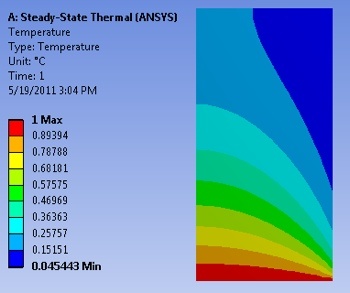
To view the temperature distribution over the surface, select Solution > Temperature from the tree on the left.
...
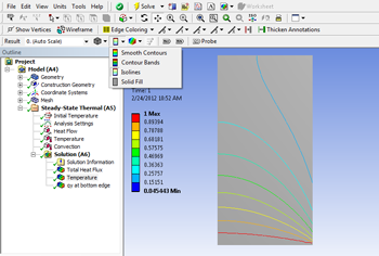
https://confluence.cornell.edu/download/attachments/146918520/UnrefTemp_Full.PNGIn order to view the contours as isolines, select the viewing button, and change from Contour Bands into Isolines.
...
https://confluence.cornell.edu/download/attachments/146918520/Isolines.pngTotal Heat Flux
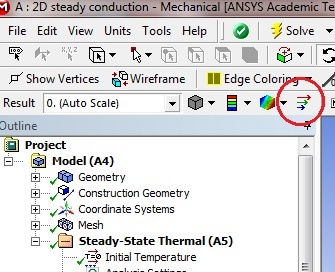
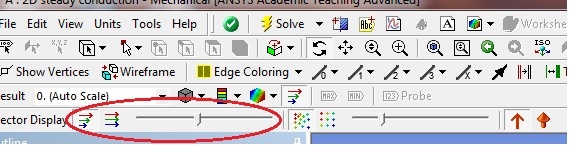
We will view the heat flux as vectors. This will tell us the direction of heat flow within the geometry as well as at the boundaries In order to plot the heat flux vectors, select Solution > Total Heat Flux from the tree on the left. Then (Click) Vectors,  near the top of the GUI. The sliders in the top bar can be used to change the size and number of vectors displayed.
At this point, the heat flux vectors should appear similar to the image below. Take a minute to think about whether the heat flow directions at the boundaries match what you expect.
...
https://confluence.cornell.edu/download/attachments/146918520/DirHeatFluxVec_Full.pngTemperature along Y=1m line
...
https://confluence.cornell.edu/download/attachments/146918520/InsConstructGeomFull.PNG...
https://confluence.cornell.edu/download/attachments/146918520/InsertPath_Full.PNG...
| Include Page | ||||
|---|---|---|---|---|
|

Temperature Contours
| HTML |
|---|
<iframe width="640" height="360" src="https://www.youtube.com/embed/LZRNtWlTZH4" frameborder="0" allowfullscreen></iframe> |
Check your Understanding
...
You then have the option to export this into a text file or an Excel file. Either will work, but for this tutorial we have exported to excel.
...
https://confluence.cornell.edu/download/attachments/146918520/PathTempResults_Full.PNGDirectional Heat Flux along Y=0m line
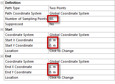
Now we are interested in calculating the heat flux through the bottom boundary. First, construct a path, following steps similar to those above, but with the start and end points at the bottom corners of the surface. (Right Click) Model > Insert > Construction Geometry. Next, (Right Click) Construction Geometry > Insert > Path. Then, set Number of Sampling Points to 200, set Start X Coordinate to 0, set Start Y Coordinate to 0, set End X Coordinate to 1, and set End Y Coordinate to 0 as shown below.
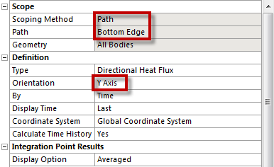
Similar to the Temperature inserted along the first path, now insert Directional Heat Flux results along Path 2. (Right Click) Solution > Insert > Thermal > Directional Heat Flux. Choose Path for the Scoping Method, set Path 2 for the Path and Y axis for Orientation, as seen below.
{neww(Click) Solve, , and ANSYS will find the Directional Heat Flux on the line y=0m as a function of x position. We would like to find the total heat flux through the bottom by integrating the flux along that boundary. To do this we will export the data to MATLAB and perform a numerical integration. Right click in the tabular data displayed in the lower righthand corner of the screen. Select all (Ctrl+A), right-click and select Export. Save the file as "qy_bot.txt" in your MATLAB working directory.
Next, open MATLAB and use the following code to integrate along the path:
clear all; clc;
qy_bot = dlmread('qy_bot.txt', '', 'B2..C50');
qy_bot_tot = trapz(qy_bot(:,1),qy_bot(:,2));
The dlmread function is used to read the data from the text file, while the trapz function performs numerical integration using trapezoids. The variable 'qy_bot_tot' calculated in MATLAB represents the total dimensionless heat flux through the bottom, y=0 line.
Save
...
Go to Step 7: Verification and Validation
See and rate the complete Learning Module& Validation