 Sign-up for free online course on ANSYS simulations!
| Include Page |
|---|
...
|
...
|
| Panel |
|---|
Author: John Singleton, Cornell University Problem Specification |
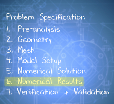
6. Results
If necessary , download the solution by right-clicking the following link: conduction 2d.zip
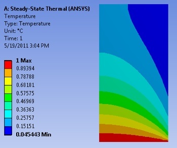
Temperature
To view the Temperature over the surface, select Solution > Temperature from the tree on the left.
...
https://confluence.cornell.edu/download/attachments/146918520/UnrefTemp_Full.PNGIn order to view the Isolines of the object, select the viewing button, and change from Contour Bands into Isolines. 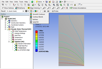
...
https://confluence.cornell.edu/download/attachments/146918520/Isolines.pngTotal Heat Flux
...
| Include Page | ||||
|---|---|---|---|---|
|
Temperature Contours
| HTML |
|---|
<iframe width="640" height="360" src="https://www.youtube.com/embed/LZRNtWlTZH4" frameborder="0" allowfullscreen></iframe> |
Check your Understanding
...
https://confluence.cornell.edu/download/attachments/146918520/DirHeatFluxVec_Full.pngTemperature along Y=1m line
...
https://confluence.cornell.edu/download/attachments/146918520/InsConstructGeomFull.PNG...
https://confluence.cornell.edu/download/attachments/146918520/InsertPath_Full.PNG...
https://confluence.cornell.edu/download/attachments/146918520/PathDet_Full.PNG...
https://confluence.cornell.edu/download/attachments/146918520/DetTemp2_Full.PNG...
https://confluence.cornell.edu/download/attachments/146918520/PathTempResults_Full.PNGDirectional Heat Flux along Y=0m line
Now we are interested in calculating the heat flux through the bottom boundary. First, construct a path, following steps similar to those above, but with the start and end points at the bottom corners of the surface. (Right Click) Model > Insert > Construction Geometry. Next, (Right Click) Construction Geometry > Insert > Path. Then, set Number of Sampling Points to 200, set Start X Coordinate to 0, set Start Y Coordinate to 0, set End X Coordinate to 1, and set End Y Coordinate to 0 as shown below.
...
https://confluence.cornell.edu/download/attachments/146918520/PathDet_Full.PNG
Similar to the Temperature inserted along the first path, now insert Directional Heat Flux results along Path 2. (Right Click) Solution > Insert > Thermal > Directional Heat Flux. Choose Path for the Scoping Method, set Path 2 for the Path and Y axis for Orientation, as seen below.
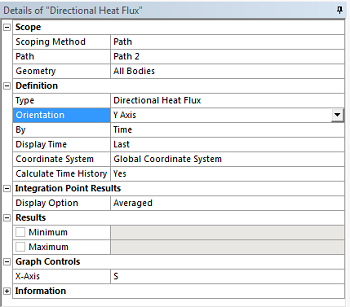
...
Now,(Click) Solve,  , and ANSYS will find the Directional Heat Flux on the line y=0m as a function of x position. We would like to find the Total Heat Flux through the bottom, by integrating the flux along that boundary. To do this we will export the data to MATLAB and perform a numerical integration. To do so, right click in the tabular data displayed in the lower righthand corner of the screen. Select all (Ctrl+A), right-click and select Export. Save the file as "qy_bot.txt" in your MATLAB working directory.
Next, open MATLAB and use the following code to integrate along the path:
clear all; clc;
qy_bot = dlmread('qy_bot.txt', '', 'B2..C50');
qy_bot_tot = trapz(qy_bot(:,1),qy_bot(:,2));
The dlmread function is used to read the data from the text file, while the trapz function performs numerical integration using trapezoids. The variable 'qy_bot_tot' calculated in MATLAB represents the total dimensionless heat flux through the bottom, y=0 line.
Save
...
Go to Step 7: Verification and Validation
See and rate the complete Learning Module& Validation