 Sign-up for free online course on ANSYS simulations!
| Include Page | ||||
|---|---|---|---|---|
|
| Include Page | ||||
|---|---|---|---|---|
|
Exercises
| Info |
|---|
MAE 3240/4230/5230: You DO NOT need to do this section. |
Exercise 1
Simulate the laminar boundary layer over a flat plate using FLUENT for a Reynolds number  where
where
Change the value of the coefficient of viscosity µ from the tutorial example to get , keeping all other parameters the same. After changing the coefficient of viscosity rerun the solver for the mesh that was created in Step 3.
...
First order boundary layer theory says that the flow outside of the boundary layer remains undisturbed, but we see that FLUENT predicts an overshoot in the velocity due to the presence of the boundary layer since the flow accelerates (For a more in depth explanation see the video explaining this here). This acceleration and overshoot can be attributed to the displacement thickness of the boundary layer. In this exercise, modify the flat plate to account for this displacement thickness, plot the velocity at the outlet, and compare your results to the flat plate solution from the tutorial.
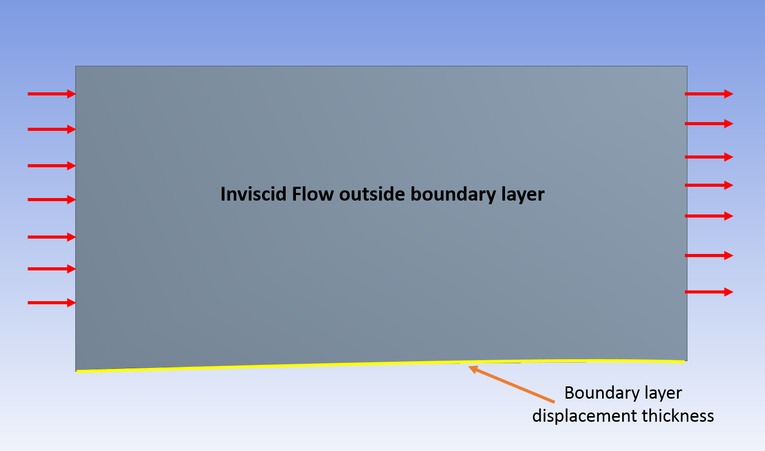
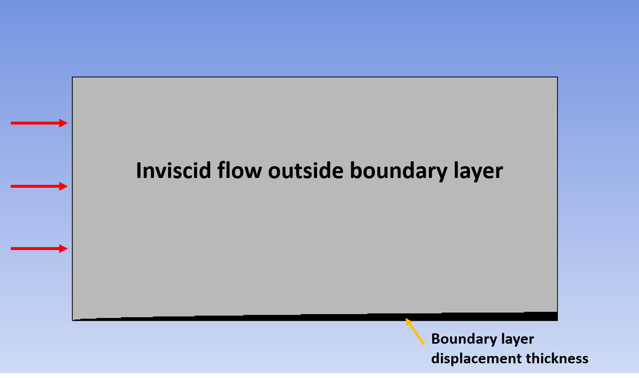
You will need to create a geometry file that can imported into DesignModeler. There are several ways to do this but one way to do so is to create the curve for the boundary layer displacement thickness in Excel and then connect the appropriate points together. Remember, DesignModeler takes in "zones" which will be your first column so that it can identify the edges in the geometry. The second column will be the points in those zones DesignModeler connects together. The third , fourth, and fifth columns are your x, y, z points respectively. Since this problem is 2D, the z column should be all 0. For a further explanation on how DesignModeler takes in this file, see here under the coordinates file explanation.
For example: if you wanted to make a square with a height and length of 1, your file would look like this:
| Zone | Point | X | Y | Z |
|---|---|---|---|---|
| 1 | 1 | 0 | 0 | 0 |
| 1 | 2 | 0 | 1 | 0 |
| 2 | 1 | 0 | 1 | 0 |
| 2 | 2 | 1 | 1 | 0 |
| 3 | 1 | 1 | 1 | 0 |
| 3 | 2 | 1 | 0 | 0 |
| 4 | 1 | 1 | 0 | 0 |
| 4 | 2 | 0 | 0 | 0 |
Flow outside of the boundary layer is inviscid and you will need to change this in your Model Setup.
Once you have run the simulation, you should see something similar to the plot below: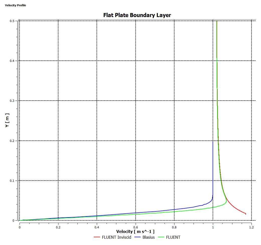
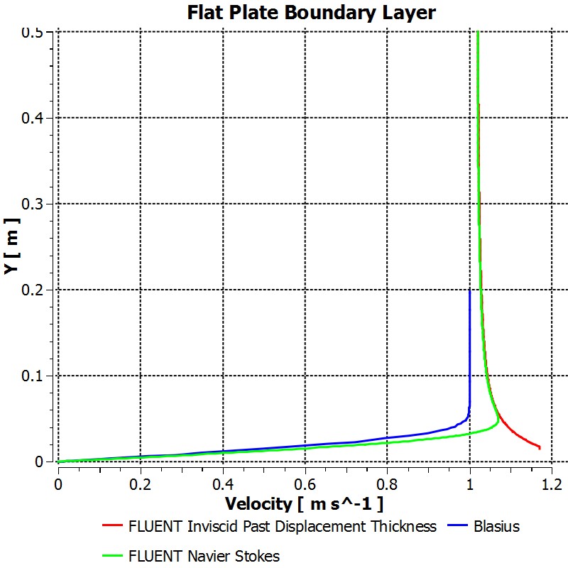
What happens to the velocity at the outlet when we account for the displacement thickness? Compare your FLUENT results from this exercise to the results from the tutorial and the Blasius solution, what is happening to the velocity profile at the outlet?