 Sign-up for free online course on ANSYS simulations!
| Include Page |
|---|
...
|
...
|
| Include Page |
|---|
...
|
...
|
| Note |
|---|
This tutorial was created with an older version of ANSYS (14.5), where the mesh generator and the refinement process was not as strong as it is now. This will result in a different solution than the one shown. (In ANSYS 16.1, the optimization results in a radius of ~1.25in-1.27in and in ANSYS 2019 R2 the optimization results in a radius of ~1.11-1.13in) |
Optimization
Set-Up of
...
Optimization
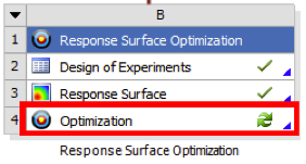
Begin this step, by double clicking on Optimization.
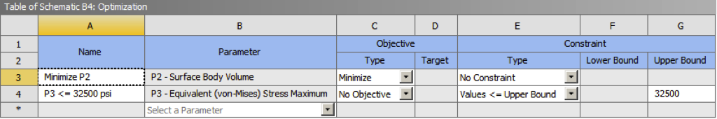
At this point, ANSYS must be told that the objective function(volume) is to be minimized while staying below the 32.5 KSI ksi Von Mises stress threshold. Under, . First, select “Objectives and Constraints” in the outline window. Then, in the "Table of Schematic B4: Optimization" change the Objective of window, select the parameter to be P2-Surface Body Volume and change the objective type to Minimize. Next, change the Objective of Equivalent Stress Maximum add in a second parameter which will be P3-Equivalent (von Mises) Stress Maximum, change the constraint type to Values <= Target. Then, set the Target Value of Equivalent Stress Maximum equal to 32,500 PSI. Upper Bound and enter 32500 for the Upper Bound. Your table should now look like the one below.
Now, execute the optimization by clicking on Update and click on Optimization from the outline window to view the results. The optimization should yield similar results to the results shown, below.
newwindow
https://confluence.cornell.edu/download/attachments/131466109/ResultsRoundOne_Full.pngModifying The Priority of The Constraints
...
The optimization tool found three candidate points that matched our given constraints and objectives. This computation was pretty fast because the optimization tool used the response surface model (plots) that previously generated. It did not actually solve our model by doing a matrix inversion. Remember that the response surface model is only an approximation of the relationship between the parameters and so our results might not be very accurate. Thankfully, we can solve our model using these candidate points to “verify” that they really do satisfy our constraints.
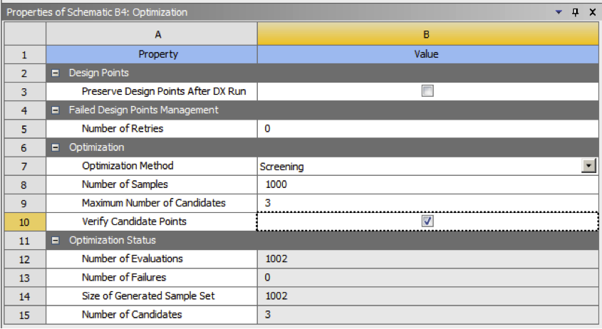
In the Properties of Schematic B4: Optimization window, insert a check to Verify Candidate Points and click on Update once again. Notice how much longer it takes to solve our model.
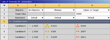
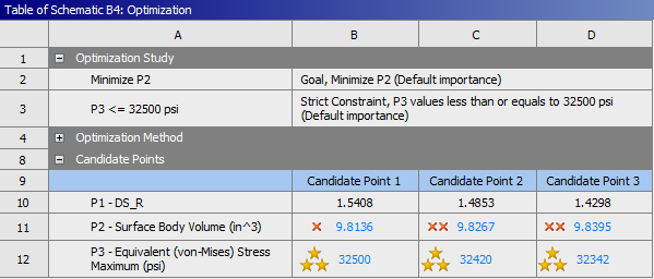
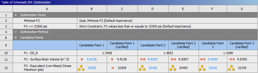
The optimization should yield similar results to the following table. Surprise! Some candidate points do not satisfy the maximum Von Mises stress constraint (now marked with a red cross). This is why it is important to always verify the candidate points.
Note: In version 2019 R2, we found that all three of the candidate points failed at this step, so don't be concerned if that is what you find.
By selecting candidate points under the results section of the Outline of Schematic B4: Optimization window, you can also see how the results of each candidate points differ from the results of a specified reference candidate point. Additionally, you can even add new candidate points.
Output parameter values calculated from simulations (design point updates) are displayed in black text, while output parameter values calculated from a response surface are dis- played in blue.
The number of gold stars or red crosses displayed next to each goal-driven parameter indicate how well the parameter meets the stated goal, from three red crosses (the worst) to three gold stars (the best).
Tip: Remember how we specified the radius to range from 1 to 2.5 inches to create the Response Surface? Well we now know that the optimized radius should be around 1.45 inches so no need to have that big of a range anymore. For a second round of optimization (not done in this tutorial), it would be a good idea to go back in Design of Experiments and change the lower and upper bounds to be, say 1.4 and 1.5 inches respectively. A smaller range will give you a more accurate response surface which will help you optimize the radius further.
Obtaining Deformation and Stress Results for Selected Design Point
We will select candidate point 2 as the design point. It is a good idea to review the deformation and stress plots at the chosen design point. To do this, let's set the radius from Candidate Point 2 as
...
https://confluence.cornell.edu/download/attachments/131466109/OptResultsRoundTwo_Full.pngObtaining the Graphical Results
At this point the Candidate A results will be inputted back into the Design Modeler. That, is the radius from Candidate A will be set as the radius of the hole in Design Modeler. In order to do so, Select (Right Click) Candidate A Point 2 > Insert as Design PointsPoint.

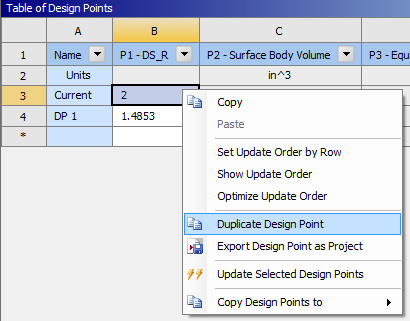
Next, click Return to Project and double click on Parameter Set. In Selecting Insert as Design Point created the design point DP1. Now in the "Table of Design Points" (Right Click) Current > Duplicate design point then design point.
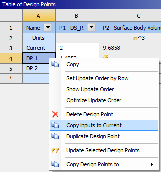
You have just duplicated the parameters from the original geometry into the new design point DP2. Now (Right Click) DP1 > Copy Inputs to Current. In the previous commands you saved the previous current design point by moving it to DP2 and you have inserted Candidate A into the Current design point. Now, click click on Update All Design Points. Now, the in the toolbar.
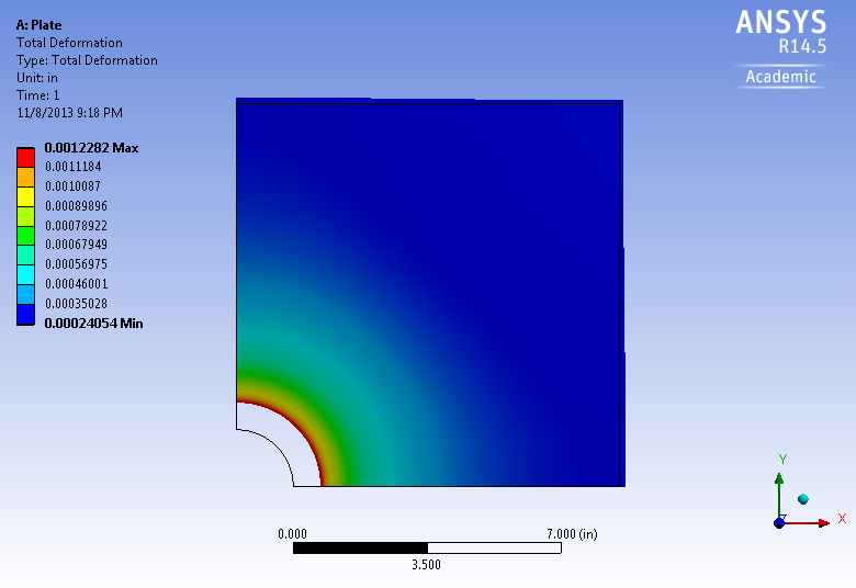
The radius of Candidate Apoint 2 has been inserted as the radius in the Design Modeler. Next, click . Let’s now view the results of our model with our optimized radius of 1.4853. Click on Return to Project and double click Results. Now, the graphical results for the Candidate A radius of 1.4725 inches can be viewed. The graphs below display the directional total deformation , and the equivalent Von Mises stress and the normal stress respectively.. You should realize that we did a fantastic job with this optimization problem! It does not get much better than this as the equivalent Von Mises stress lies just under our constraint. Well...not really. Let's take a look at the verification and validation step.
Total Deformation
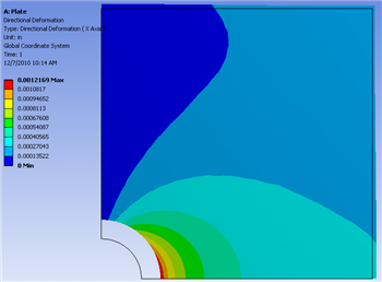
 Directional Deformation (X Direction)
newwindow
Equivalent Von Mises Stress 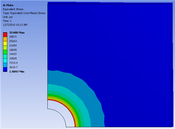
newwindow
https://confluence.cornell.edu/download/attachments/131466109/EquivStress_RoundTwo_InitMesh_Full.png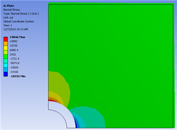
https://confluence.cornell.edu/download/attachments/131466109/NormStress_RoundTwo_InitMesh_Full.png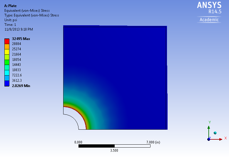
Go to Step 7: Verification & ValidationSee and rate the complete Learning Module