 Sign-up for free online course on ANSYS simulations!
| Include Page | ||||
|---|---|---|---|---|
|
| Include Page | ||||
|---|---|---|---|---|
|
Numerical Results
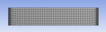
Before we explore the ANSYS results, let's take a peek at the mesh.
...
Click on Mesh (above Solution ) in the tree outline. This shows the mesh used to generate the ANSYS solution. The domain is a rectangle. This domain is discretized into a number of small "elements". Recall that ANSYS solves the BVP and calculates the displacements at the nodes. A finer mesh is used near the left and right ends where we expect greater stress concentration. We have checked that the solution presented to you is reasonably independent of the mesh.
Units
Set the units for the results display by selecting Units > Metric (mm, kg, N, s, mV, mA) . The displacements will be reported in mm and the stresses in N/mm2 which is equivalent to MPa.
...
The stresses are derived from the nodal displacements using Hooke's law. In the following video, we look at the sigma_x distribution in the interior and at the boundaries and compare the ANSYS values to the values expected from the analytical solution and traction boundary conditions.
| HTML |
|---|
| Wiki Markup |
{html}<iframe width="600" height="338" src="//www.youtube.com/embed/vBNFUYrsWMw?rel=0" frameborder="0" allowfullscreen></iframe>{html} |
Summary of the above video investigating sigma_x:
- Click on probe and hover over the bar. Using the probe may tell you the stress associated with a specific point on the bar.
- To view the less noticeable stress contours, click on the scale to edit. In this video, the orange (2nd highest value) was changed to 250 and the blue (2nd lowest value) was changed to 50. The contour map changed to display the subtle difference in sigma_x.
In the video, we saw that ANSYS's values for sigma_x matches with:
...
- The value away from the boundaries is close to zero as expected from the analytical solution. It is not exactly zero because of round-off errors.
- The value at the top and bottom boundaries are close to zero. This agrees with the boundary condition at these boundaries since the traction has to be zero at these free boundaries. In other words, the normal component of the traction acting on these surfaces is sigma_y and that has to be zero since the traction on these free surfaces is zero.
- There is significant deviation from the analytical solution at both ends. The analytical solution breaks down at these ends because of the additional assumptions that we made. Note that there are areas where sigma_y is negative i.e. compressive.
tau_xy
We expect tau_xy to be zero away from the ends. Near the ends, since sigma_x and sigma_y are non-zero, we expect
| Latex |
|---|
\begin{align*} |
| Wiki Markup |
{latex} \[ \tau_{xy} = \tau_{xy}(x,y) \] end{latexalign*} |
Plot tau_xy, look at the range of values and use Probe to check actual values. Are the above statements valid?
Equivalent Stress (Von Mises):
The Equivalent or Von Mises stress is used to predict yielding of the material. We can see that the analytical solution under-predicts the maximum equivalent stress. Thus, one would need to use a large factor of safety if using the analytical result while designing such a structure. One would use a factor of safety with the FEA result also but it does not have to be as large.
Go to Step 3: Verification and Validation
...