 Sign-up for free online course on ANSYS simulations!
Results:
| Include Page |
|---|
...
|
...
|
...
Again, it must be stressed that the mesh, geometry, boundary conditions and solver steps have been skipped in this exercise. You are instead given the solutions to the aforementioned problem simulated by ANSYS workbench. You are encouraged to explore these results and understand the different underlying assumptions of the analytical 1D Boundary Value Problem compared to the ANSYS 2D Boundary Value Problem. As you will see, the analytical approach can successfully account for the stresses in the middle of the bar, but fails to accurately model stresses at the point load and end effects.
...
Mesh:
...
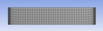
The figure above depicts the mesh used to generate the results you see below. The domain is rectangle. Please note that although this problem has been solved using discrete elements, it is not uniformly discretized. A finer mesh is used in areas of predicted greater stress concentration. We want to be able to accurately simulate the end effects of the bar.
...
Displacement:
...
| Include Page | ||||
|---|---|---|---|---|
|
Numerical Results
Before we explore the ANSYS results, let's take a peek at the mesh.
Mesh
Click on Mesh (above Solution ) in the tree outline. This shows the mesh used to generate the ANSYS solution. The domain is a rectangle. This domain is discretized into a number of small "elements". Recall that ANSYS solves the BVP and calculates the displacements at the nodes. A finer mesh is used near the left and right ends where we expect greater stress concentration. We have checked that the solution presented to you is reasonably independent of the mesh.
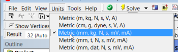
Units
Set the units for the results display by selecting Units > Metric (mm, kg, N, s, mV, mA) . The displacements will be reported in mm and the stresses in N/mm2 which is equivalent to MPa.
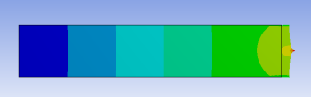
Displacement
To view the deformed structure, click on Solution > Displacement in the tree outline. The black rectangle shows the undeformed structure. The deformed structure is colored by the magnitude of the displacement. The displayed displacement distribution is calculated by interpolating the nodal displacements. Red areas have deformed more and blue areas less. You can see that the left end has not moved as specified in the problem statement. This means this boundary condition has been applied correctly. The displacement increases from left to right as we intuitively expect. There is also not much variation in the y-direction. So we can conclude that the model has been constrained properly.
Note the extremely high deformation near the point load. This extremum is unrealistic and should be ignored (there are no point loads in reality).
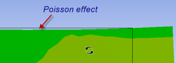
To view the Poisson effect (shrinking in the y direction), zoom into the top-rightright corner by drawing a rectangle around the region with the right mouse button.

You can do this multiple times to zoom in more. You do indeed see the shrinking in the y-direction as expected but it is small for this model.
You can restore the front view of the entire model by right-clicking in the background and choosing View > Front .
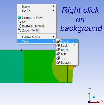
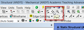
Note that you can zoom in and out using the middle mouse wheel. You can translate the model by clicking on the Pan button and dragging the model with the left mouse button. There are also a bunch of zoom options next to the Pan button.
sigma_x
The stresses are derived from the nodal displacements using Hooke's law. In the following video, we look at the sigma_x distribution in the interior and at the boundaries and compare the ANSYS values to the values expected from the analytical solution and traction boundary conditions.
| HTML |
|---|
<iframe width="600" height="338" src="//www.youtube.com/embed/vBNFUYrsWMw?rel=0" frameborder="0" allowfullscreen></iframe> |
Summary of the above video investigating sigma_x:
- Click on probe and hover over the bar. Using the probe may tell you the stress associated with a specific point on the bar.
- To view the less noticeable stress contours, click on the scale to edit. In this video, the orange (2nd highest value) was changed to 250 and the blue (2nd lowest value) was changed to 50. The contour map changed to display the subtle difference in sigma_x.
In the video, we saw that ANSYS's values for sigma_x matches with:
- The analytical solution in the interior (away from the left and right boundaries)
- Traction boundary condition for sigma_x at the right boundary
Note that sigma_x at the location of the point load is infinite. So as the mesh is refined further, sigma_x at the point load will get larger and larger without bound.
sigma_y
Next, let's take a look at sigma_y. Click on Solution > sigma_y in the tree outline. Again, probe values in the middle as well as at the ends. Check that:
- The value away from the boundaries is close to zero as expected from the analytical solution. It is not exactly zero because of round-off errors.
- The value at the top and bottom boundaries are close to zero. This agrees with the boundary condition at these boundaries since the traction has to be zero at these free boundaries. In other words, the normal component of the traction acting on these surfaces is sigma_y and that has to be zero since the traction on these free surfaces is zero.
- There is significant deviation from the analytical solution at both ends. The analytical solution breaks down at these ends because of the additional assumptions that we made
...
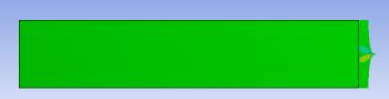
Sigma_x:
...
Note here that the stress in x direction is not constant as assumed in the analytical method. If we were to pick a section near the middle of the bar, our analytical result would be nearly accurate. The solution, however, no longer applies when considering the stresses at the wall, and the stresses near the point load. Obviously, the stresses in the x-direction maximizes at the point load.
...
Sigma_y:
...
- . Note that there are areas where sigma_y is negative
...
- i.e. compressive.

tau_xy
We expect tau_xy to be zero away from the ends. Near the ends, since sigma_x and sigma_y are non-zero, we expect
| Latex |
|---|
\begin{align*}
\tau_{xy} = \tau_{xy}(x,y)
\end{align*} |
Plot tau_xy, look at the range of values and use Probe to check actual values. Are the above statements valid?
Equivalent Stress (Von Mises):
The Equivalent or
...
Tau_xy:
...
Von Mises:
...
Von Mises stress is used to predict yielding of the material. We can consider see that the analytical solution under-predicts the maximum and minimum von mises stress as the critical design points. For example, in this case, we would want to design our beam with reference to the area around the point load to prevent reaching limit load of the material anywhere on the bar. 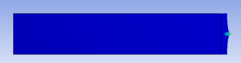
...
...
equivalent stress. Thus, one would need to use a large factor of safety if using the analytical result while designing such a structure. One would use a factor of safety with the FEA result also but it does not have to be as large.
Go to Step 3: Verification and Validation See and rate the complete Learning Module