Page History

...

Click Display.

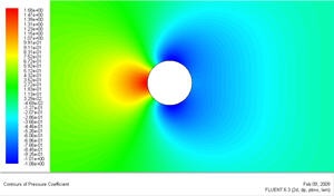
Because the cylinder is cylindricalsymmetry in shape, we see that the pressure coefficient profile is symmetry between the top and bottom of cylinder.

...

Display > Contours

Under Contours of, choose PressureVelocity.. and Pressure Coefficient Stream Function. Select Deselect the Filled option. Increase the number of contour levels plotted: set Levels to 100. Click Display.

Image AddedBecause the cylinder is cylindrical, we see that the pressure coefficient profile is symmetry between the top and bottom of cylinder

Let's set the reference values necessary to calculate the pressure coefficient.

Report > Reference Values

Select farfield under Compute From.

Image Removed

The above reference values of density, velocity and pressure will be used to calculate the pressure coefficient from the pressure. Click OK.

Display > Contours...

Select Pressure... and Static Pressure from under Contours Of. Then select Pressure Coeffient.

Image Removed
(Click picture for larger image)

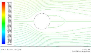
The pressure coefficient after the shockwave is 0.293, very close to the theoretical value of 0.289. The pressure increases after the shockwave as we would expectEnclosed streamlines at the back of cylinder clearly shows the recirculation region.
Go to Step 7: Verify Results

...