 Sign-up for free online course on ANSYS simulations!
Step 6: Analyze Results
Plot Velocity Vectors
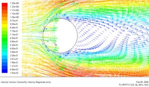
Let's plot the velocity vectors obtained from the FLUENT solution.
Display > Vectors
Set the Scale to 14 and Skip to 4. Click Display.
| newwindow | ||||
|---|---|---|---|---|
| ||||
| Wiki Markup | ||||
{panel} Author: Rajesh Bhaskaran & Yong Sheng Khoo, Cornell University [Problem Specification|FLUENT - Steady Flow Past a Cylinder - Problem Specification]\\ [1. Create Geometry in GAMBIT|FLUENT - Steady Flow Past a Cylinder - Step 1]\\ [2. Mesh Geometry in GAMBIT|FLUENT - Steady Flow Past a Cylinder - Step 2]\\ [3. Specify Boundary Types in GAMBIT|FLUENT - Steady Flow Past a Cylinder - Step 3]\\ [4. Set Up Problem in FLUENT|FLUENT - Steady Flow Past a Cylinder - Step 4]\\ [5. Solve|FLUENT - Steady Flow Past a Cylinder - Step 5]\\ {color:#ff0000}{*}6. Analyze Results{*}{color}\\ [7. Refine Mesh|FLUENT - Steady Flow Past a Cylinder - Step 7]\\ [Problem 1|FLUENT - Steady Flow Past a Cylinder - Problem 1]\\ [Problem 2|FLUENT - Steady Flow Past a Cylinder - Problem 2] {panel} h2. Step 6: Analyze Results h4. Plot Velocity Vectors Let's plot the velocity vectors obtained from the FLUENT solution. *Display > Vectors* Set the {color:#660099}{*}{_}Scale{_}{*}{color} to 14 and {color:#660099}{*}{_}Skip{_}{*}{color} to 4. Click {color:#660099}{*}{_}Display{_}{*}{color}. \\ [!step6_velocity_vectorsm.jpg!|^step6_velocity_vector.jpg] {newwindow:Higher Resolution Image}https://confluence.cornell.edu/download/attachments/104400192/step6_velocity_vector.jpg?version=1{newwindow} |
From
...
this
...
figure,
...
we
...
see
...
that
...
there
...
is
...
a
...
region
...
of
...
low
...
velocity
...
and
...
recirculation
...
at
...
the
...
back
...
of
...
cylinder.
| Info | ||||||||||||||||||||
|---|---|---|---|---|---|---|---|---|---|---|---|---|---|---|---|---|---|---|---|---|
| =
|
|
|
|
|
|
|
|
| |||||||||||
Pressure Coefficient
Pressure coefficient is a dimensionless parameter defined by the equation  where p is the static pressure, p ref is the reference pressure, and q ref is the reference dynamic pressure defined by
| Latex |
|---|
\large $$} {info} h4. Pressure Coefficient Pressure coefficient is a dimensionless parameter defined by the equation !step6_cp_equation.gif! where _p_ is the static pressure, _p_ ~ref~ is the reference pressure, and _q_ ~ref~ is the reference dynamic pressure defined by {latex}\large && q_{ref} = {1 \over 2} {\rho_{ref}v_{ref}^2} $${latex} \\ The reference $$ |
The reference pressure,
...
density,
...
and
...
velocity
...
are
...
defined
...
in
...
the
...
Reference
...
Values
...
panel
...
in
...
Step
...
5.
...
Let's
...
plot
...
pressure
...
coefficient
...
vs
...
x-direction
...
along
...
the
...
cylinder.
...
Plot
...
>
...
XY
...
Plot...
...
Change
...
the
...
Y
...
Axis
...
Function
...
to
...
Pressure
...
...
...
,
...
followed
...
by
...
Pressure
...
Coefficient
...
.
...
Then,
...
select cylinder under Surfaces.
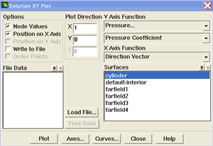
Click Plot.
| newwindow | ||||
|---|---|---|---|---|
| ||||
https://confluence.cornell.edu/download/attachments/104400192/step6_Cpplot.jpg?version=1 |
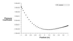
As can be seen, the pressure coefficient at the back is lower than the pressure coefficient at the front of the cylinder. The irrecoverable pressure is due to the separation at the back of cylinder and the frictional loss.
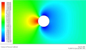
Now, let's take a look at the Contour of Pressure Coefficient variation around the cylinder.
Display > Contours
Under Contours of, choose Pressure.. and Pressure Coefficient. Select the Filled option. Increase the number of contour levels plotted: set Levels to 100.
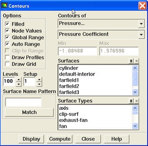
Click Display.
| newwindow | ||||
|---|---|---|---|---|
| ||||
https://confluence.cornell.edu/download/attachments/104400192/step6_Cp_contour.jpg?version=1 |
Because the cylinder is symmetry in shape, we see that the pressure coefficient profile is symmetry between the top and bottom of cylinder.
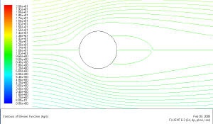
Plot Stream Function
Now, let's take a look at the Stream Function.
Display > Contours
Under Contours of, choose Velocity.. and Stream Function. Deselect the Filled option. Click Display.
| newwindow | ||||
|---|---|---|---|---|
| ||||
https://confluence.cornell.edu/download/attachments/104400192/step6_streamline.jpg?version=1 |
Enclosed streamlines at the back of cylinder clearly shows the recirculation region.
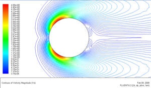
Plot Vorticity Magnitude
Let's take a look at the Pressure Coefficient variation around the cylinder. Vorticity is a measure of the rate of rotation in a fluid.
Display > Contours
Under Contours of, choose Velocity.. and Vorticity Magnitude. Deselect the Filled option. Click Display.
| newwindow | ||||
|---|---|---|---|---|
| ||||
https://confluence.cornell.edu/download/attachments/104400192/step6_vorticity.jpg?version=1 |