 Sign-up for free online course on ANSYS simulations!
Step 6: Analyze Results
Plot Velocity Vectors
Let's plot the velocity vectors obtained from the FLUENT solution.
Display > Vectors
Under Color by, select Mach Number in place of Velocity Magnitude since the former is of greater interest in compressible flow. The colors of the velocity vectors will indicate the Mach number. Use the default settings by clicking Display.
This draws an arrow at the center of each cell. The direction of the arrow indicates the velocity direction and the magnitude is proportional to the velocity magnitude (not Mach number, despite the previous setting). The color indicates the corresponding Mach number value. The arrows show up a little more clearly if we reduce their lengths. Change Scale to 0.2. Click Display.
Zoom in a little using the middle mouse button to peer more closely at the velocity vectors.
(Click picture for larger image)
We can see the flow turning through an oblique shock wave as expected. Behind the shock, the flow is parallel to the wedge and the Mach number is 2.2. Save this figure to a file:
Main Menu > File > Hardcopy
Select JPEG and Color. Uncheck Landscape Orientation. Save the file as wedge_vv.jpg in your working directory. Check this iimage by opening this file in an image viewer.
Let's investigate how many mesh cells it takes for the flow to turn. Tturn on the mesh by clicking on the Draw Grid checkbox in the Vectors menu. In the Grid Display menu that pops up, click Display. This displays the mesh in the graphics window. Close the Grid Display menu. Click Display in the Vectors menu. Zoom in further as shown below.
(Click picture for larger image)
We see that it takes 2-3 mesh cells for the flow to turn. According to inviscid theory, the shock is a discontinuity and the flow should turn instantly. In the FLUENT results, the shock is "smeared" over 2-3 cells. In the discrete equations that FLUENT solves, there are terms that act like viscosity. This introduced viscosity contributes to the smearing. A more thorough explanation would have to go into the details of the numerical solution procedure.
Plot Mach Number Contours
Set the Scale to 14 and Skip to 4. Click Display.
| newwindow | ||||
|---|---|---|---|---|
| ||||
https://confluence.cornell.edu/download/attachments/104400192/step6_velocity_vector.jpg?version=1 |
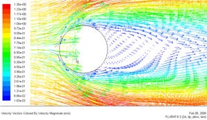
From this figure, we see that there is a region of low velocity and recirculation at the back of cylinder.
| Info | ||
|---|---|---|
| ||
Pressure Coefficient
Pressure coefficient is a dimensionless parameter defined by the equation  where p is the static pressure, p ref is the reference pressure, and q ref is the reference dynamic pressure defined by
| Latex |
|---|
\large $$ q_{ref} = {1 \over 2}{\rho_{ref}v_{ref}^2}$$ |
The reference pressure, density, and velocity are defined in the Reference Values panel in Step 5.
Let's plot pressure coefficient vs x-direction along the cylinder.
Plot > XY Plot...
Change the Y Axis Function to Pressure..., followed by Pressure Coefficient. Then, select cylinder under Surfaces.
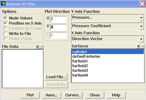
Click Plot.
| newwindow | ||||
|---|---|---|---|---|
| ||||
https://confluence.cornell.edu/download/attachments/104400192/step6_Cpplot.jpg?version=1 |
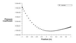
As can be seen, the pressure coefficient at the back is lower than the pressure coefficient at the front of the cylinder. The irrecoverable pressure is due to the separation at the back of cylinder and the frictional loss.
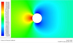
Now, let's take a look at the Contour of Pressure Coefficient variation around the cylinderLet's take a look at the Mach number variation in the flowfield.
Display > Contours
Under Contours of, choose Velocity Pressure.. and Mach Number Pressure Coefficient. Select the Filled option. Increase the number of contour levels plotted: set Levels to 100.
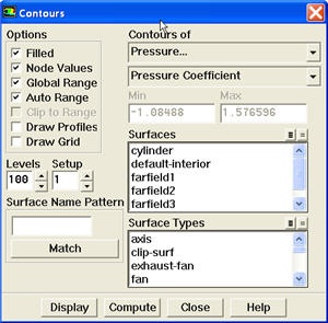
Click Display.
(Click picture for larger image)
We see that the Mach number behind the shockwave is uniform and equal to 2.2. Compare this to the corresponding analytical result.
Plot Pressure Coefficient Contours
Let's set the reference values necessary to calculate the pressure coefficient.
Report > Reference Values
Select farfield under Compute From.
The above reference values of density, velocity and pressure will be used to calculate the pressure coefficient from the pressure. Click OK.
Display > Contours...
Select Pressure... and Static Pressure from under Contours Of. Then select Pressure Coeffient.
(Click picture for larger image)
The pressure coefficient after the shockwave is 0.293, very close to the theoretical value of 0.289. The pressure increases after the shockwave as we would expect.
| newwindow | ||||
|---|---|---|---|---|
| ||||
https://confluence.cornell.edu/download/attachments/104400192/step6_Cp_contour.jpg?version=1 |
Because the cylinder is symmetry in shape, we see that the pressure coefficient profile is symmetry between the top and bottom of cylinder.
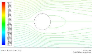
Plot Stream Function
Now, let's take a look at the Stream Function.
Display > Contours
Under Contours of, choose Velocity.. and Stream Function. Deselect the Filled option. Click Display.
| newwindow | ||||
|---|---|---|---|---|
| ||||
https://confluence.cornell.edu/download/attachments/104400192/step6_streamline.jpg?version=1 |
Enclosed streamlines at the back of cylinder clearly shows the recirculation region.
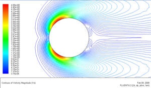
Plot Vorticity Magnitude
Let's take a look at the Pressure Coefficient variation around the cylinder. Vorticity is a measure of the rate of rotation in a fluid.
Display > Contours
Under Contours of, choose Velocity.. and Vorticity Magnitude. Deselect the Filled option. Click Display.
| newwindow | ||||
|---|---|---|---|---|
| ||||
https://confluence.cornell.edu/download/attachments/104400192/step6_vorticity.jpg?version=1 |
Go to Step 7: Refine MeshGo to Step 7: Verify Results