 Sign-up for free online course on ANSYS simulations!
| Include Page |
|---|
...
|
...
|
| Panel |
|---|
Author: John Singleton and Rajesh Bhaskaran Problem Specification |
...
| Include Page | ||||
|---|---|---|---|---|
|
Physics Setup
...
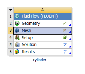
Your workbench project page should look like this.
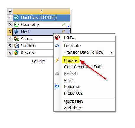
We are done with all the meshing steps but for some reason, a tick mark doesn't appear next to Mesh in the project page. To get the tick mark next to mesh, right-lick click on it and select Update as shown below.
Launch Fluent
(Double Click) Setup in the Workbench Project Page.
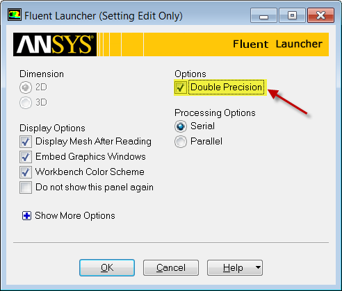
Double Precision
Select Double Precision.
Parallel Processing
If you are using a computer that has more than one core, it is advantageous to turn on the parallel processing feature of FLUENT when the mesh gets large. This feature will divide the solution domain amongst the number of cores that you specify. The maximum number of cores that you can specify is 4 for the standard FLUENT package. The Swanson Lab at Cornell University has dual core machines. If you want to use both cores, set Processing Options to Parallel (Local Machine) and set the Number of Processes to 2. These selections are shown below. For this problem, you might not get much speedup by using both cores. So you could also leave it at the default of "Serial" which will use one core.

If you have more cores set Number of Processes to the number of cores you have ( 4 is the limit). Now, when you run your calculations in FLUENT you will have more than one core working for you, which will significantly reduce your computation time. Lastly, click OKWhen the FLUENT Launcher appears change options to "Double Precision", and then click OK as shown below.The Double Precision option is used to select the double-precision solver. In the double-precision solver, each floating point number is represented using 64 bits in contrast to the single-precision solver which uses 32 bits. The extra bits increase not only the precision, but also the range of magnitudes that can be represented. The downside of using double precision is that it requires more memory.
Twiddle your thumbs a bit while the FLUENT interface starts up. This is where we'll specify the governing equations and boundary conditions for our boundary-value problem. On the left-hand side of the FLUENT interface, we see various items listed under Problem Setup. We will work from top to bottom of the Problem Setup items to setup the physics of our boundary-value problem. On the right hand side, we have the Graphics pane and, below that, the Command pane.
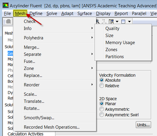
Check Mesh
(Click) Mesh > Info > Size
You should now have an output in the command pane stating that there are 18,432 cells.
(Click) Check > Perform Mesh > Check
You should see no errors in the command pane.
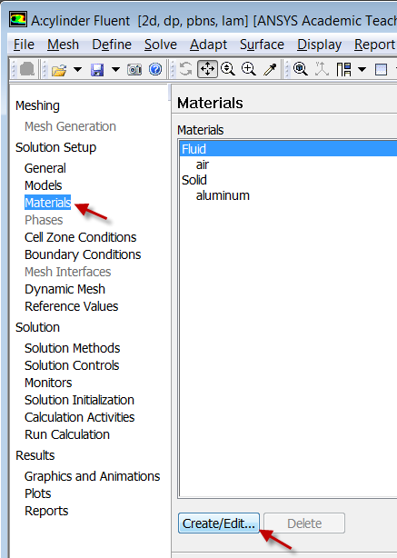
Specify Material Properties
Problem Solution Setup > Materials > Fluid > Create/Edit....
Then set the Density to 1 kg/m^3 and set Viscosity to 0.05 kg/m*s. Click Change/Create then click Close.
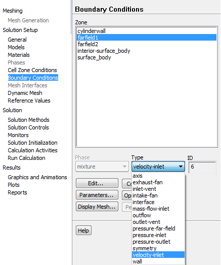
Boundary Conditions
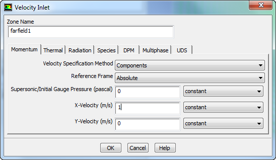
FarField1
Problem Solution Setup > Boundary Conditions > farfield1.
Set Type to velocity-inlet. Click Edit.... Set Velocity Specification Method to Components, set X-Velocity to 1 m/s, and set Y-Velocity to 0 m/s.
FarField2
Problem Solution Setup > Boundary Conditions > farfield2..
Set Type to pressure-outlet.
...
Cylinder Wall
...
Note that pressures in the FLUENT interface are specified in terms of gauge values where: gauge pressure = absolute pressure - reference pressure. The reference pressure is 1 atm by default. So in our case the gauge pressure at the outlet is 0 atm which is also the default. The following video from the laminar pipe flow module in our free online course explains the advantages of working in terms of gauge pressures. The video discusses this in the context of laminar pipe flow but the same ideas apply for our cylinder flow too.
| HTML |
|---|
<iframe width="560" height="315" src="https://www.youtube.com/embed/83J4kNC3Fyg?ecver=2" frameborder="0" allowfullscreen></iframe> |
Cylinder Wall
Solution Problem Setup > Boundary Conditions > cylinderwall.
Set Type to wall.This is the default.
Reference Values
Problem Solution Setup > Reference Values.
Set the Density to 1 kg/m^3. The other default values will work for the purposes of this simulation.
Save Project
Go to Step 5: Solution
See and rate the complete Learning ModuleNumerical Solution