The information on this page pertains to the research performed by the Spring 2010 Inlet Manifold team. See Sedimentation Tank Hydraulics for the most up-to-date research.
Objectives
The objectives of this research team are to experimentally test the inlet manifold recreating the same conditions that will face in a real AguaClara plant, and modify the design based on the results.
To begin with, we calculated the manifold dimensions which include:
- Pipe diameter
- Ports' diameter
- Ports' spacing
The calculations for this experiment were based on the Agalteca design flow and tank dimensions.
Based on the Manifold Theory, the initial idea is to prove that to create an evenly distributed flow throughout the different ports of the manifold, we would have to taper the pipe to have the same velocity along the manifold and therefore the same flow in each port.
To begin with the study, the idea is to prove that a constant diameter manifold would fail to deliver an evenly distrubuted flow along the ports. Therefore we should calculate a manifold with a constant diameter for the design flow and the desired velocity which should be higher than 0.15 m/s (minimum scour velocity). To calculate the manifold diameter we use the following equation and round diameter to a commercial drill size:
Unable to find DVI conversion log file.With the rounded Diameter, we calculated the real velocity inside the manifold using the following equation:
Unable to find DVI conversion log file.Now by changing the distance between ports (
Unable to find DVI conversion log file.) and we can calculate the amount of ports (
Unable to find DVI conversion log file.) needed, different ports' diameters (
Unable to find DVI conversion log file.) and also energy dissipation rates (
Unable to find DVI conversion log file.) through those ports, by using the following equations:
Unable to find DVI conversion log file.Number of ports we can calculate the flow per port
Unable to find DVI conversion log file.Once we calculated the flow we can calculate the port's area and diameter
Unable to find DVI conversion log file. Unable to find DVI conversion log file.Finally the energy dissipation rate should be checked to ensure that the flocs will not break while entering the Sedimentation Tank.
These two equations are equivalents. The first equation was derived from Monroe and the second one was provided by him also from external bibliography.
Unable to find DVI conversion log file. Unable to find DVI conversion log file.The results of those calculation proposed a 6" PVC pipe with 1" ports spaced 5 cm center to center (total 57 ports). Drilling Process Images
These calculations assumed that the sum of the areas of the vena contracta of the ports should equal the cross sectional area of the pipe. The justification of this assumption is based on the following graph, where we can see how the flow distribution varies along the manifold, as the ratio of the manifold cross sectional area and the sum of the areas of the vena contracta of the ports (from now on expressed as Am/Avc ratio) varies.
Figure 2: Am/Avc ratio graph
By looking at this graph, it is clear that the best flow distribution would be having an Am/Avc ratio of 3. There are two ways to have this relationship and these are:
- Have a very large diameter manifold
- Have very small ports' diameteres
Both these solutions will create unwanted scenarios.
- The velocities inside the manifold will be too slow. Possible sludge settling inside the manifold. Also the idea is to make this design adequate for larger plant flows, with the consequence of having too large of a pipe inside the sedimentation tank which is not desirable.
- The energy dissipation rate of the flow coming out of the ports will be too high leading to potential floc breakup.
Based on these the next best flow distribution is when the Am/Avc ratio is 1 and in these case we daon't have the unwanted scenarios just described so it is reasonable to proceed with this Am/Avc ratio.
The next step is to recreate in the lab the conditions of that manifold in the Agalteca plant. To do this, a submersible pump with the design flow will recreate the inlet flow and the whole manifold replica, will be installed in a flume to begin the flow testing.
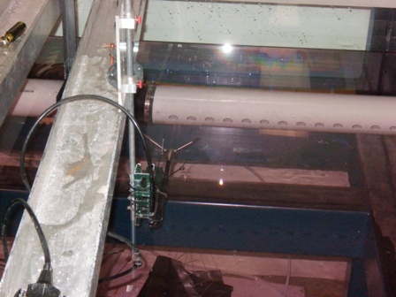
The of the ports will be measured using an ADV as shown in the following image.
The results obtained by this measurements will be plotted and compared to the theoretical expected values.
Based on the obtained results, the manifold should be modified and the testing procedure should be repeated until even flow distribution is achieved.
Experimental Methods and Results
Setup and Procedure
Unknown macro: {float}
Unable to render embedded object: File (ManifoldStraight.png) not found.
Figure 3: Manifold running parallel to the flume wall and bed
The manifold we designed is a 10' long, 6" PVC pipe with 1" diameter holes drilled every 5cm. The manifold had water pumped through it at a rate of 3.8 L/sec (roughly 1 gallon/min) and the water flows through a whole 10' section of 6" PVC pipe before it gets to the manifold to ensure that the effects of the pump have dissipated in the pipe. The manifold is suspended 14" above the bed of the flume by U-clamps and the manifold is spaced 7" from the flume wall to make sure that it runs parallel to the flume bed and wall. We double checked this by measuring the distance from the flume wall and flume bed both at the beginning of the manifold and at the end of the manifold. The ports of the manifold are positioned so that the jets exiting from them run parallel to the bottom of the tank.
The Acoustic Doppler Velocimeter (ADV) used to take velocity readings was mounted to a beam running across the width of the flume. The ADV was positioned so that it was aimed head on into the ports (so it also lies parallel to the bed of the flume) at a fixed distance of 17 cm from the port openings.
Unknown macro: {float}
Unable to render embedded object: File (ExampleVelocityProfile.png) not found.
Figure 4: Example of a velocity profile of one of the ports
The measurements were taken every 5-6 ports, which gave us 10 different data points along the manifold. For each port, we maneuvered the ADV to the edge of the port hole. We then took measurements as we moved the ADV across the port in steps of 0.5cm. We recorded data for approximately 1 minute and then moved the ADV 0.5cm further and measured again until we were sure we had captured the entire jet profile.
In the analysis of our data, we took the mean of the velocities at each port. Then we plotted the velocity profile for each port and estimated the maximum flow rate at each port. These calculations were then plotted along the length of the manifold to give a velocity profile for the each manifold setup.
Results
Experiment 1: 10' Uniform Manifold Am/Avc=1
Experiment 2: 10' Uniform Manifold Am/Avc=1, take 2
Experiment 3: 20' Uniform Manifold Am/Avc=0.5
Experiment 4: 10' Uniform Manifold Am/Avc=0.5
Experiment 5: Manifold Cross-Sectional Measurements