 Sign-up for free online course on ANSYS simulations!
UNDER CONSTRUCTION
Author: Daniel Kantor and Andrew Einstein, Cornell University
Problem Specification
1. Create Geometry in GAMBIT
2. Mesh Geometry in GAMBIT
3. Specify Boundary Types in GAMBIT
4. Set Up Problem in FLUENT
5. Solve!
6. Analyze Results
7. Refine Mesh
Problem 1
Step 6: Analyze Results
For all of our analysis we will be looking at the Sphere surface under Surfaces, unless otherwise noted.
Plot Velocity Vectors
Let's plot the velocity vectors obtained from the FLUENT solution.
Display > Vectors
Set the Scale to 14 and Skip to 4. Click Display.
[!step6_velocity_vectorsm.jpg!|^step6_velocity_vector.jpg]
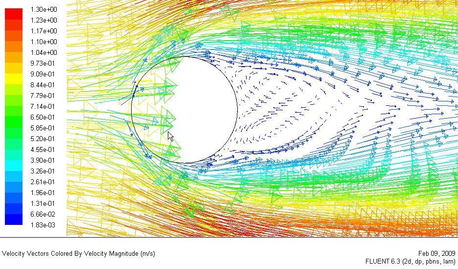
*******From this figure, we see that there is a region of low velocity and recirculation at the back of cylinder.**************
Zoom in the cylinder using the middle mouse button.
Now, let's take a look at the Contour of Pressure Coefficient variation around the cylinder.
Display > Contours
Under Contours of, choose Pressure.. and Pressure Coefficient. Select the Filled option. Increase the number of contour levels plotted: set Levels to 100.
Unable to render embedded object: File (step6_Cphowto.jpg) not found.
Click Display.
[!step6_Cp_contoursm.jpg!|^step6_Cp_contour.jpg]
*********Because the cylinder is symmetry in shape, we see that the pressure coefficient profile is symmetry between the top and bottom of cylinder.********
Plot Stream Function
Now, let's take a look at the Stream Function.
Display > Contours
Under Contours of, choose Velocity.. and Stream Function. Deselect the Filled option. Click Display.
[!step6_streamlinesm.jpg!|^step6_streamline.jpg]
**********Enclosed streamlines at the back of cylinder clearly shows the recirculation region.************
Plot Vorticity Magnitude
Let's take a look at the Pressure Coefficient variation around the Sphere. Vorticity is a measure of the rate of rotation in a fluid.
Display > Contours
Under Contours of, choose Velocity.. and Vorticity Magnitude. Deselect the Filled option. Click Display.
[!step6_vorticitysm.jpg!|^step6_vorticity.jpg]
Pressure Coefficient
Pressure coefficient is a dimensionless parameter defined by the equation Unable to render embedded object: File (step6_cp_equation.gif) not found. where p is the static pressure, p ref is the reference pressure, and q ref is the reference dynamic pressure defined by
Unknown macro: {latex}
\large $$ q_
Unknown macro: {ref}
=
Unknown macro: {1 over 2}
{\rho_
v_
Unknown macro: {ref}
^2}$$
The reference pressure, density, and velocity are defined in the Reference Values panel in Step 5.
Let's plot pressure coefficient vs x-direction along the cylinder.
Plot > XY Plot...
Change the Y Axis Function to Pressure..., followed by Pressure Coefficient. Then, select Sphere under Surfaces.
Unable to render embedded object: File (Step6_CpPanel.png) not found.
Click Plot.
[!step6_Cpplotsm.jpg!|^step6_Cpplot.jpg]
We see that there is a lot of scatter in our data, so we will be creating a line along the sphere to try and get a better picture of the pressure coefficient.