Verification & Validation

Verification

Adapt the Mesh

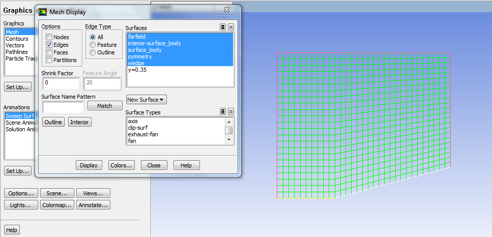
In order to test our simulation for convergence, we will refine the mesh. Refining the mesh will allow use to make sure that the results we are calculating are independent of the mesh. However, instead of refining the mesh everywhere (which would be wasteful, as most of the area of the domain far away from the shock has constant values), we will use our results to refine our mesh. Specifically, we are going to use the gradient of the pressure to determine where to refine the mesh. First, let's take a look at our mesh. In the Outline window, select Graphics and Animations, under _Graphics, select Mesh, then press Setup. Select all of the surfaces (except y=0.35) and press Display. This will display the current mesh.

You may now close the Mesh Display window. In the menu bar, go to Adapt > Gradient. Under Options uncheck Coarsen. Ensure that Gradients of > Pressure... Static Pressure are selected. Then press Compute.

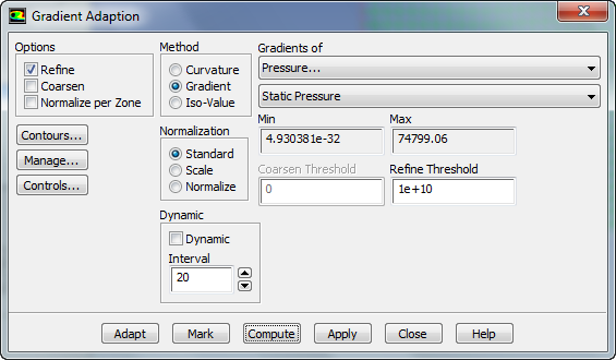
This will compute the maximum and minimum gradients of static pressure. Next, we need to pick a threshold. In order to do this, click on Contours.... This will open the familiar Contours window. In the Contours window, select Contours of Adaption... Existing Value, then press Compute. This will populate the Contours menu with the values were were viewing for adaption, in this case, gradient of the static pressure. Also, make sure to uncheck Node Values.

Finally, press Display to display the contours of static pressure gradient.

For every element that has a pressure above that threshold, that element will be refined. Let's make our threshold 10000. Enter 10000 into Refine Threshold. Then press Adapt. You will be asked if you want to change the mesh. Press Yes.

It will seem like nothing has changed, but that is because we need to re-display the mesh in order to see the adaption. The new mesh should look something like this.

Notice that the area surrounding the shock was refined. Now, re-initialize the solution, (Solution Initialization > Compute From Farfield > Initialize), and rerun the solution (you will also need to increase the number of iterations – I recommend 3000).

Now, once again, plot the contours of the mach number. Below is a comparison of the mach number results from the original mesh and the refined mesh.

Original Mesh

Refined Mesh

The most striking difference between the two results is the thickness of the shock. Notice that for the refined mesh, the shock is less thick that for the original mesh. This shows that the refined mesh is converging towards the real case.

Comparison to Analytical Solution

In order to verify our simulation, we need to compare our results to either an analytical solution or an experiment. Below is a table comparing the values from the simulation with the calculations from the pre-analysis.

As we can see from the table, we are getting fairly good matching between the computation and analytical approaches. From this we can build our trust in our simulation.

Continue to Exercises