Page History

...

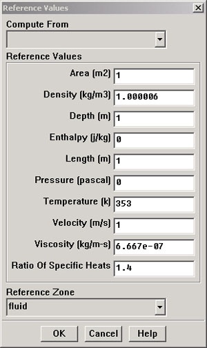
Select inflow under Compute From to tell FLUENT to use values at the inflow for the reference values. Check that the reference value for velocity is 1 m/s, temperature is 353 K, and coefficient of viscosity is 6.667e-7 kg/m-s as given in the Problem Specification. These reference values will be used to non-dimensionalize the distance of the cell center from the wall to obtain the corresponding y+ values. Click OK.

By using the following method, plot y+ values for wall-adjacent cells to check how they compare with the recommendation mentioned above.

...

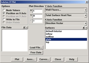
Make sure that Position on X Axis is set under Options, that 1 is the value next to X, and 0 is the value next to Y under Plot Direction. Recall that this tells FLUENT to plot the x-coordinate value on the abscissa of the graph. Select Turbulence... under Y Axis Function and select Wall Yplus from the drop down list under that. Since we want the y+ value for cells adjacent to the wall of the pipe, choose plate under Surfaces.

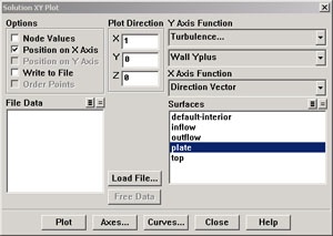
Click Plot.

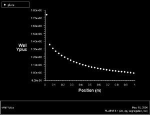
(Click picture for larger image)

...

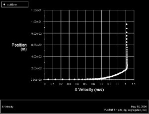
Under X Axis Function, pick Velocity... and then in the box under that, pick X Velocity. Finally, select outflow under Surfaces since we are plotting the velocity profile at the outflow. De-select plate under Surfaces.

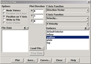
Click on Axes... in the Solution XY Plot window. Select X in the Axis box. In the Options box select Major Rules to turn on the grid lines in the plot. Click Apply. Then select the Y in the Axis box, select Major Rules again, and turn off Auto Range. In the Range box enter 0.1 for the Maximum so that we may view the velocity profile in the boundary layer region more closely. Click Apply and Close.

...

Uncheck Write to File. Click Plot.

 
(Click picture for larger image)

We notice here that the x velocity reaches 1 m/s at approximately y = 0.02 m. This shows the relative thinness of the boundary layer compared to the length scale of the plate. We also notice that the velocity profile is slightly greater than 1 m/s above the boundary layer. We know this would not happen in real flow, rather it is a result of the boundary condition we have chosen for our model. We chose the Symmetryboundary condition at the top of our flow field, which is essentially a wall without the no-slip condition. Thus, no flow is permitted to escape through this boundary.

In a real external flow, there is no such boundary at the top and flow is permitted to pass through freely. When we consider the inflow and outflow velocity profiles in terms of conservation of mass, the uniform velocity profile of 1 m/s at x = 0 has more mass entering the flow field than the non-uniform velocity profile at x = 1m, in which the velocity is lower near the plate. In addition, the fluid is expanding near the plate because its temperature is increasing, further increasing the y-velocity of the fluid above it. These factors require that some mass must escape through the top of our flow field in order to satisfy conservation of mass.

 
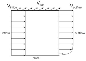
Choosing a Pressure Outlet for the top boundary condition would represent real external flow more accurately. Unfortunately, this cannot be used in our flow field without encountering convergence problems, so selecting the Symmetry boundary condition was the next best option. Because we are not allowing flow to escape through the top boundary, we observe an outflow velocity profile in which outflow velocity is greater than 1 above the boundary layer in order to satisfy conservation of mass. Fortunately, the inaccuracies resulting from the model we chose have no significant effect on the heat transfer coefficients at the plate.

...

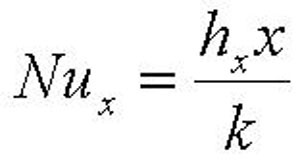
Recall that the Nusselt Number is a non-dimensional heat transfer coefficient that relates convective and conductive heat transfer.

 
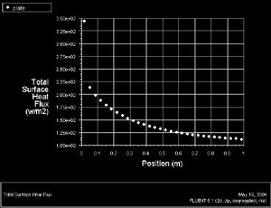
In order to obtain the Nusselt Number from FLUENT, we will begin by plotting Total Surface Heat Flux.

...

In the Options box, change back to Position on X Axis. In the Plot Direction box, enter the default values of 1 in the X box and 0 in the Y box. Under Y-Axis Function choose Wall Fluxes. In the box below, chose Total Surface Heat Flux. Select Plate under Surfaces. Before plotting, be sure to turn on Auto Range for the Y axis under Axes....

 
Click Plot.

 
(click picture for larger image)

...

Open the file heatflux.xy using Wordpad or a similar application. You can simply copy and paste the data into Excel.

 
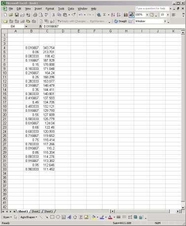
If Excel does not automatically separate the data into columns, separate it by selecting the column of data and then using the Text to Columns function:

...

The first column is the x location on the plate and the second column is the total surface heat flux (q'') at the corresponding x location. We now need to determine the Nusselt number from these values at each x location. We will define positive q'' as heat transfer into the fluid. Use the following expression to convert q'' to Nusselt Number in your Excel spreadsheet.

 
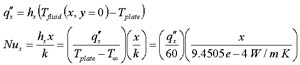
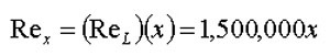
Reynolds Number can be defined at each x location by

 
Now plot Re vs. Nu in Excel. Your plot should look like this:

 
(click picture for larger image)

...

Validate your results form FLUENT by comparing to a correlation and experimental results. The correlation we will use is derived by Reynolds \[1\]: !06_reynolds.jpg!
 
All properties in this correlation are evaluated at the free-stream static temperature of 300K.This correlation assumes the 

Image Added
 
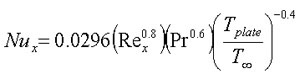
All properties in this correlation are evaluated at the free-stream static temperature of 300K.This correlation assumes the following:

1. Pr = 0.7

2. 10^5 < Re < 10^7

...

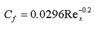
6. Friction factor calculated from the following relation (implicit in Nu equation above, does not need to be calculated in your analysis):

 
Add the Reynolds correlation for Nusselt Number to your Excel spreadsheet.

Seban & Doughty \[2\] performed a heated flat plate experiment for which they derived the following expression for Nusselt Number: !06_Seban_experiment2.jpg!
 
The Seban & Doughtyexperiment was performed with air as the fluid (Pr = 

Image Added
 
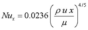
The Seban & Doughty experiment was performed with air as the fluid (Pr = 0.7) and at various Reynolds Numbers in the range 1e5 < Re < 4e6. Add the this experimental relation for Nusselt Number to your Excel spreadsheet.

Now plot and compare Re vs. Nu from FLUENT, the Reynolds Correlation, and Seban's experiment.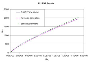
 (click picture for larger image)

As we can see, there is very little variation between these 3 results. The largest % error between the FLUENT results and the Reynolds correlation is only 7.5%. In turbulent flow as we have here, similar results between FLUENT and correlation are more difficult to come by than in laminar flow because a turbulent model must be used in FLUENT, which does not solve the Navier-Stokes Equations exactly. Experimental error (in experiments from which correlations are derived) also accounts for some of this 7.5% error. Each of the turbulence models that FLUENT offers produces results similar to these, although the k-epsilon model is the most appropriate model to use in this case.

...