Page History

...

This brings up the Contour Nodal Solution Data menu. Select Stress from the left list, von Mises SEQV from the right list and click OK. Zoom in at the point of contact.

Image Added

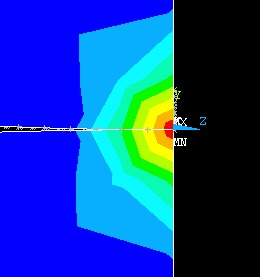
The contour plot also shows the locations of the maximum and minimum values with the labels MX and MN, respectively. As you can see, the upper and lower disks have deformed and come into contact.

...

This brings up the List Nodal Solution menu. Select Stress from the left list, Principals SPRINOK from the right and click OK .

The first three columns list the first, second and third principal stresses at each node. Scroll all the way down in this window.

Image Added
 

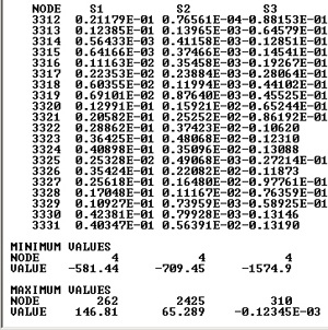
As you can see, the maximum principal stress is -1574.9. Recall that the the applied force was specified in Newtons (p=4500N) and the geometry in mm. As a result, the max principal stress has units of N/mm². Also note that the value is negative, which tells us that the max stress is a compressive stress. This is what one would expect based on the loading conditions.

...

This brings up the List Nodal Solution menu. Select DOF solution from the left list, Translation UY from the right and click OK.

Image Added
 

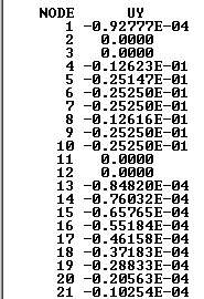
The approach can be determined by finding the total displacement of a node attached to the upper surface of the upper disk. Since all the nodes attached to the upper area will be equally displaced as a result of the coupled boundary condition, we can look at the displacement of any node attached to the upper surface.

...