Page History

Step

...

As discussed in the previous step, we'll first mesh the subsection AEFG that we just created.

Set Mesh Size Along Edges

We'll use the previously-defined parameters NDIV_X, NDIV_Y and SIZE_Z to set the mesh size along edges. The table below describes what each parameter is and the value we have assigned to it.

6: Specify boundary conditions

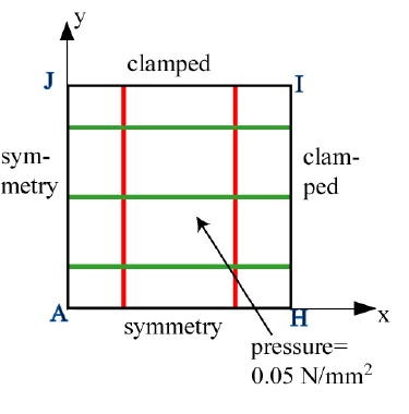
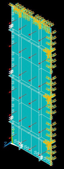
The boundary conditions given in the problem specification are summarized in the schematic below. Keep in mind that the edge conditions need to be applied to the plate as well as the stiffeners.

Image Added

Apply Symmetry along AH

We'll apply this BC in two steps:

1. Select edges along AH
2. Apply symmetry condition to the selected edges

Plot areas: Utility Menu > Plot > Areas

Adjust the display: Click on the Isometric View and Fit View icons in the rightmost part of the GUI.

Utility Menu > PlotCtrls > Numbering: Turn off area and node numbering; turn on line numbering.

Select all edges along AH: Utility Menu > Select > Entities

...

Parameter

...

Value

...

Description

...

NDIV_X

...

3

...

No. of divisions for edges along x

...

NDIV_Y

...

6

...

No. of divisions for edges along y

...

SIZE_Z

...

5

...

Size of divisions for edges along z

...

We are going to continually use the

...

Select Entitiesmenu to

...

apply the

...

BC's. So resize and rearrange the windows slightly so that you can access this menu, the

...

ANSYS GUI, and the tutorial simultaneously.

...

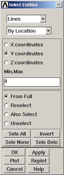
Select Entities menu: Select Lines from the pull-down menu at the top. Select below that. Choose By LocationY coordinates. Under Min,Max, enter 0. This will select all lines whose centers lie at y=0. Make sure From Full is selected so that we are selecting entities from the full model. Click Apply.

Image Added

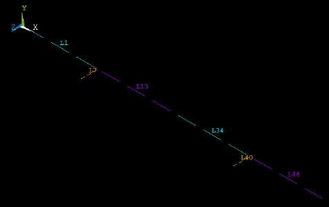
Check which lines have been selected: Select Entities menu >Plot. You should see that the edges along AH have been selected.

Image Added

Apply symmetry condition to the selected edges: Main Menu > Preprocessor > Loads > Define Loads > Apply > Structural > Displacement > Symmetry B.C. > On Lines > Pick All

This applies the symmetry condition to all the selected lines.

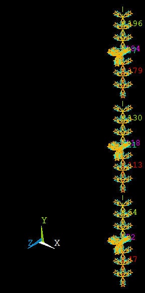
Select the entire model: Click Select All and then Replot in the Select Entities menu. You should see the S symbol along the edges where the symmetry BC has been applied.

Apply Symmetry along AJ

We'll first select all edges along AJ. Go back to Select Entities menu: Leave Lines and By Location in place. Choose X coordinates. Under Min,Max, retain 0. This will select all lines whose centers lie at x=0. Make sure From Full is selected. Click Apply.

Check which lines have been selected: Select Entities menu > Replot. You should see that only the edges along AJ are currently selected.

Let's apply the symmety BC to these edges: Main Menu > Preprocessor > Loads > Define Loads > Apply > Structural > Displacement > Symmetry B.C. > On Lines > Pick All

Select the entire model: Click Select All and then Replot in the Select Entities menu.

Apply Clamped BC along HI

Now that we've gotten the hang of this boundary business, let's mop up Operation BC's in short order.

Select Entities menu: Leave Lines, By Location and X coordinates selections in place. Under Min,Max, enter W1. This will select all lines whose centers lie at x=W1. Make sure From Full is selected. Click Apply.

Select Entities menu > Replot

Constrain all six nodal degrees of freedom (DOF) for the selected edges:Main Menu > Preprocessor > Loads > Define Loads > Apply > Structural > Displacement > On Lines > Pick All > All DOF > OK

The (cluttered) display will show that all six DOF's have been constrained.

Image Added

Select Entities menu: Select All and Replot

Apply Clamped BC along JI

Select Entities menu: Leave Lines, and By Location in place. Choose Y coordinates. Under Min,Max, enter L1. This will select all lines whose centers lie at y=L1. Make sure From Full is selected. Click Apply.

Select Entities menu > Replot

Constrain all six nodal degrees of freedom (DOF) for selected edges:Main Menu > Preprocessor > Loads > Define Loads > Apply > Structural > Displacement > On Lines > Pick All > All DOF > OK

Select Entities menu: Select All and Replot

Save: Toolbar > SAVE_DB

Apply Pressure on Plate

Utility Menu > PlotCtrls > Numbering: Turn off line numbering.

Utility Menu > Plot > Areas

Choose areas corresponding to the plate: In the Select Entities menu, select Areas from the pull-down menu at the top. Leave By Location below that. Choose Z coordinates Under Min,Max, enter 0. This will select all areas whose centers lie at z=0. Make sure From Full is selected. Click Apply.

Check which areas are currently selected: Select Entities menu > Replot

Apply a pressure of 0.05 N/mm² on the plate in the +z direction: Main Menu > Preprocessor > Loads > Define Loads > Apply > Structural > Pressure > On Areas > Pick All

For VALUE, enter 0.05. Click OK.

ANSYS will mark the faces where the pressure is applied. Let's instead plot the applied pressure using arrows to check its direction: Utility Menu > PlotCtrls > Symbols. For Surface Load Symbols, select Pressures and under Show pres and convect as, select Arrows. Click OK. Are the pressures acting in the right direction?

Select Entities menu: Select All, Replot and Cancel. You should now see the entire model. Review that all the BC's have been applied correctly.

Image Added

Save: Toolbar > SAVE_DB

Create Log File

In parametric studies to be undertaken later, we'll start with the log file containing the commands from the first six steps that we just went through. To save this log file, select

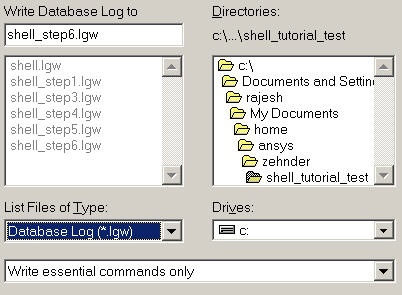
Utility Menu > File > Write DB log file

Under Write Database Log to, enter the filename for the logfile: shell_step6.lgw. At the bottom of this menu, select Write Essential Commands only. Click OK. Review shell_step6.lgw by opening it in a text editor.

Image Added

Go to Step 7: Solve!

See and rate the complete Learning Module

Go to all ANSYS Learning Modules

Generate Mesh for Plate

Recall that the plate and the horizontal and vertical stiffeners have different thicknesses which have been assigned to different "real constant" sets. Jog your memory about which thicknesses have been assigned to which "real constant" sets in Step 2.
We'll first mesh the plate using real constant set #1. Under Element Attributes in MeshTool, click on Set. You will see that the element type and material number are already set and the default real constant set is #1. These are the options we need for the plate; so these don't need to be changed. Click Cancel.
Plot areas: Utility Menu > Plot > Areas
Click on Mesh in MeshTool. Pick area A1 and click OK. The resulting mesh for the plate is displayed.

Generate Mesh for Vertical Stiffener

Under Element Attributes in MeshTool, click on Set. Set Real constant set number to 2 and click OK.
Plot areas: Utility Menu > Plot > Areas
Click on Mesh in MeshTool. Pick area A2 and click OK. The resulting mesh for the plate is displayed.

Generate Mesh for Horizontal Stiffener

Under Element Attributes, click on Set. Set Real constant set number to 3 and click OK.
Plot areas: Utility Menu > Plot > Areas
Click on Mesh in MeshTool. Pick areas A3 and A4 and click OK.
Let's change the graphical display so that the geometry is displayed as a solid model with the shell thicknesses shown. At the command prompt, type /eshape, 1 and then select Utility Menu > Plot > Replot. When the /ESHAPEcommand in issued, ANSYS uses the real constants associated with each element to determine its shape. (Note that commands are not case-senstive.)
Do the relative thicknesses of different parts of the shell look correct? Feel free to manipulate the graphical display to check this.
You can access different model views such as front, right, isometric etc. using the buttons to the right of the graphics window. At the bottom of this row of icons is the Dynamic Model Mode . Clicking this icon allows you to manipulate the model using the mouse (alternatively, you can hold down the Ctrl key). To see the help page on this mode, right-click on the icon and select Dialog Overview > Pan, Zoom, Rotate > Dynamic Mode: Model.
Save: Toolbar > SAVE_DB

Copy Mesh in x-Direction

...

• Turn on node numbers (in addition to keypoint and area numbers) using Utility Menu > PlotCtrls > Numbering
• Display elements and nodes together: Utility Menu > PlotCtrls > Multi-Plot Ctrls > OK. Leave only Nodes and Elements turned on and click OK. Select Utility Menu > Plot > Multi-Plots.
• Zoom into the bottom-center of the model as in the snaphsot below. At the bottom of the symmetry plane, you should notice that there are actually two nodes, 2 and 172. Node 2 is associated with the original area and node 172 with the copy. We'll merge coincident nodes a little later. (Note that your node numbers may be different from mine since numbering can vary on different computer systems.)

  Copy Mesh in y-Direction

  Plot areas: Utility Menu > Plot > Areas
  Click on the Fit View and Isometric View icons in the rightmost part of the GUI.
  Copy areas: Main Menu > Preprocessor > Modeling > Copy > Areas
  Pick A1, A2, and A5 and click OK.
  Copy Areas menu: Leave Number of copies as 2. For Y-offset, enter L1/(2*NSY); delete X-offset; leave Z-offset blank and click OK.
  Check the resulting mesh for sub-section ABCD: Utility Menu > Plot > Elements
  Turn-off node numbers to reduce clutter.

  Copy Sub-Section ABCD

  How many copies of sub-sectionABCD do we need to make in the x- and y-directions? What are the values of X-Offset and Y-Offset in each case? Jot your answers down so that you can check the values below.
  Copy areas: Main Menu > Preprocessor > Modeling > Copy > Areas > Pick All
  Copy Areas menu: Number of copies = NSX; X-offset = W1/NSX; Y- and Z-offsets should be blank or zero. Click Apply.
  Repeat copy in y-direction: Select Pick All again in the pick menu.
  Copy Areas menu: Number of copies = NSY; Y-offset = L1/NSY; X- and Z-offsets should be blank or zero. Click OK.
  Check the resulting mesh: Utility Menu > Plot > Elements

  Merge Coincident Entities

  We saw earlier that the copy operations resulted in coincident nodes, keypoints, etc. along shared boundaries. We need to merge these coincident items so that separate portions of the model are combined into one. Otherwise, the various portions will live as independent entities and loads applied to one portion will not be transferred to its neighbors. The effect of the merge operation is shown schematically below.
  View documentation about the merge utility: ANSYS Help > Contents > Modeling and Meshing Guide > Number Control and Element Reordering > Number Control
  This section has useful information about merging entities. It indicates that one can either merge keypoints, nodes, etc. individually or merge allcoincident entities at once (with ANSYS ensuring that they are merged in the proper sequence). Since we'd like to palm off as much work as possible to ANSYS, we'll use the latter option.
  Select Main Menu> Preprocessor> Numbering Ctrls> Merge Items
  For Type of item to be merged, select All and click OK. This will merge all coincident entities.
  Earlier we saw that nodes 2 and 172 were coincident. Zoom in on this region again with node numbers turned on. What do you see?
  If you performed the merge operation correctly, you'll see that the higher numbered node has been deleted and the two coincident nodes have been replaced by a single node.
  Save: Toolbar > SAVE_DB

  Compress Item Numbers

  If you scroll down the help section on numbering that we've been peeking at, you'll find a useful spiel on Compressing Item Numbers(section 11.1.2): "As you build your model, you might, by deleting, clearing, merging, or performing other operations, create unused slots in the numbering sequence for various items. These slots will remain empty for some items (such as elements) but will be filled in for other items (such as keypoints) as new items are created. To save data storage space (by eliminating otherwise empty numbers) or to preserve desired sequencing (by forcing newly-created items to be assigned numbers greater than those of existing items), you can eliminate these gaps by "compressing" your numbering".
  Check the range of node numbers before compressing the numbering: Utility Menu > List > Nodes > OK
  Compress numbering for all items (nodes, elements, etc.): Main Menu> Preprocessor> Numbering Ctrls> Compress Numbers
  For Item to be compressed , select All and click OK.
  Re-check the range of node numbers after compressing. You should find that the range of node numbers is reduced since there are now no gaps in the numbering.
  Close MeshTool.
  Save: Toolbar > SAVE_DB
  Go to Step 6: Specify boundary conditions

...

Copyright 2006.
Cornell University
Sibley School of Mechanical and Aerospace Engineering.

ANSYS Short Course-Tutorial List |