 Sign-up for free online course on ANSYS simulations!
| Include Page | ||||
|---|---|---|---|---|
|
| Include Page | ||||
|---|---|---|---|---|
|
| Panel |
|---|
Problem Specification |
...
Plot σx vs. ri
...
(Take 2)
Vectorize σx Calculation
Again, we pick MATLAB's brain on vectorization:
Wiki Markup
Go through the example. We'll vectorize our program by replacing loops with array operations. Since the syntax for array operations very closely resembles that for corresponding scalar operations, let's create our program starting from beam.m rather than loopy beam2.m.
Select beam.m in the Editor by clicking on its name at the bottom.
Editor (tab) > File Save > Save As
Enter beam3.m for filename. Confirm that you are editing beam3.m.
MATLAB's vectorization example shows you how you can create the vector ri using the : operator. Let's check how we can use this animal. At the command prompt, type
0.5:0.1:1.5
You can see that this creates a row vector with the first and last elements being 0.5 and 1.5, respectively. Each successive element is incremented by 0.1. The general format is start:increment:end.
...
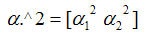
We now come to a key idea about vectorization. In the succeeding statment statement for calculating I, we have the term ri^4. To understand how MATLAB interprets it, consider the following simple example of how MATLAB interpets the ^ operator for matrices:
...
So it tries to do a matrix multiplication with α. It'll of course hiss and stamp its feet in complaint when it tries to multiply a 1x2 matrix with itself. But we are not looking for a matrix multiplication. We'd like each element to be raised to the given power viz.
Note that this is achieved by preceding the ^ operator with the period character (.). The period character can be used with other arithmetic operators such as * and /. Chew over this as it is a subtle but powerful feature. For more info, see
Help > Search Home (tab) > Documentation (icon) > Search for:) elementwise > Arthimetic Operator: arithmetic operators > Arithmetic Operators + - * / \ ^ '
So in the I statement, we replace ri^4 with ri.^4

What should we do in the succeeding sigma_x statement to vectorize it? When you try to divide by I, MATLAB will try a matrix operation. So we strategically employ our period character:
...
How do your values of sigma_x correspond to the values from beam2.m? Mine are the same ... yipppee!
Plot σx vs. ri: Take 2
Recycle the plot section from our program in Step 3. Copy this section and append it to your current program:
...
Save and run to create the plot. Let's make this plot spiffy enough that it can be included in a formal report that you submit to your boss. This can be done by expanding this section as shown below:
%Plot sigma_x vs. ri
figure(1); %Create figure #1
clf; %Clear current figure
h=plot(1e2*ri,sigma_x,'-r');
set(gca,'Box','on','LineWidth',2,...
'FontName','Helvetica',...
'FontSize',14);
%Set axis properties
set(h,'LineWidth',2);
%Set linewidth for curve
xlabel('r_i (cm)');
ylabel('\sigma_x at O (MPa)');
title('Bending stress');
axis square; %Make axis box square
We'll soon see what each of these statements does. For now, replace the plot section in your program with the above code snippet using copy-and-paste.
...
To see the effect of each statement in this code segment, let's step through it using the debugger. Close you figure window. Let's pause the execution at the figure(1) statement by setting a "breakpoint" at this statement: click in the column between the statement and the line number. A red dot will appear in this column as below.
...
Execute this statement by clicking on the step icon ![]() in icon
in icon  in the Editor. This should bring up the Figure 1 window. Note that the green arrow moves to the next statement indictating indicating that execution is paused there.
Click again on the step icon. clf will clear anything in the current figure i.e. figure 1. This means you start with a clean slate.
...
Keep an eye on the axes lines and labels in your figure as you step through the set(gca,...) command. Did you see that this command changed the font and line styles for the axes? gca stands for get current axes handle; once we have the handle, we can manipulate the axes properties (yup, same as my office). You can use this statement after any plot command; if you have multiple plot commands for the same figure, this statement needs to be used only once.
Now we will make the curve in the plot thicker. Keep an eye on the σx curve as you step through the set(h,...) statement. Did you notice a change in the line style?
Retain an eye on your figure as you step through the remaining statements. You should end up, as below, with a nice-looking plot with legible lines and text. The axis square statement makes the current axis box square in size.
...
Exit debug mode by clicking on the ![]() icon the
icon the  icon in the Editor.
See my entire program here (opens in a new windowright click and select save target as).
I strongly suggest that you be environmentally friendly and recycle the above plot commands to produce good quality figures. Since I am a nice guy, I have summarized this below as a "plot template" for your convenience; you can copy-and-paste and modify this code snippet in your future programming endeavors.
figure(1); %Create figure #1
clf; %Clear current figure
h=plot(,,'');
set(gca,'Box','on','LineWidth',2,...
'FontName','Helvetica',...
'FontSize',14);
%Set axis properties
set(h,'LineWidth',2);
%Set linewidth for curve
xlabel('');
ylabel('');
title('');
axis square; %Make axis box square
Go to Step 5: Plot σx σx vs. ri, ri (Take 3: File Input/OutputSee and rate the complete Learning Module)