 Sign-up for free online course on ANSYS simulations!
| Include Page | ||||
|---|---|---|---|---|
|
| Include Page | ||||
|---|---|---|---|---|
|
Exercises
Exercise 1: Vertical Channel Flow
Problem Specification (pdf file)
Exercise 2: Laminar Flow within Two Rotating Concentric Cylinders
Contributed by Prof. John Cimbala and Matthew Erdman, The Pennsylvania State University
Problem Specification (pdf file)
The video below shows how to use ANSYS Fluent to set up and solve a problem like this.
| HTML |
|---|
<iframe width="560" height="315" src="https://www.youtube.com/embed/3DnLP9-UruA?rel=0" frameborder="0" allowfullscreen></iframe> |
Exercise 3:
| Panel |
|---|
Problem Specification |
| Note | ||
|---|---|---|
| ||
We are working on updating this part of the tutorial. Please come back soon. |
Exercise 1
Laminar Pipe Flow
Consider developing flow in a pipe of length L = 8 m, diameter D = 0.2 m, ρ = 1 kg/m3 , µ =2 × 10⁻³ 10^−3 kg/m s, and entrance velocity uin u_in = 1 m/s (the conditions from the FLUENT case considered in classspecified in the Problem Specification section). Use FLUENT with the "second-order upwind" scheme for momentum to solve for the flowfield on meshes of 100 × 5, 100 × 10 and 100 × 20 (axial points divisions × radial pointsdivisions). The mesh files can be downloaded from Blackboard.
1. Plot the axial velocity profiles at the exit obtained from the three meshes. Also, plot the corresponding velocity profile obtained from fully-developed pipe analysis. Indicate the equation you used to generate this profile. In all, you should have four curves in a single plot. Use a legend to identify the various curves. Axial velocity u should be on the abscissa and r on the ordinate.
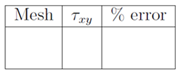
2. Calculate the shear stress τxy Tau_xy at the wall in the fully-developed region for the three meshes. Calculate the corresponding value from fully-developed pipe analysis in HW6. For each mesh, calculate the % error relative to the analytical value. Include your
results as a table:
3. At the exit of the pipe where the flow is fully-developed, we can define define the error in the centerline velocity as
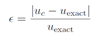
where uc u_c is the centerline value from FLUENT and uexact u_exact is the corresponding exact (analytical) value. We expect the error to take the form
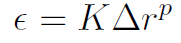
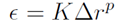
where the coefficient coefficient K and power p depend upon the order of accuracy of the discretization. Using MATLAB, perform a linear least squares fit of

to obtain the coefficients p and K. Plot ϵ vs. ∆r (using symbols) on a log-log plot. Add a line corresponding to the least-squares fit to this plot.
...
Hint: To interpret your results, you should keep in mind that the first or second-order upwind discretization applies only to the inertia terms in the momentum equation. The discretization of the viscous terms is always second-order accurate.
Return To Problem Specification