 Sign-up for free online course on ANSYS simulations!
| Include Page | ||||
|---|---|---|---|---|
|
| Include Page | ||||
|---|---|---|---|---|
|
| Info |
|---|
This module is from our free online simulations course at edX.org (sign up here). The edX interface provides a better user experience, so we have moved the module there. |
Laminar Pipe Flow
Created using ANSYS 16.2
Learning Goals
In this module, you'll learn to:
- Develop the numerical solution to a laminar pipe flow problem in ANSYS Fluent
- Verify the numerical results from ANSYS Fluent
- Connect the ANSYS steps to concepts covered in the Computational Fluid Dynamics section
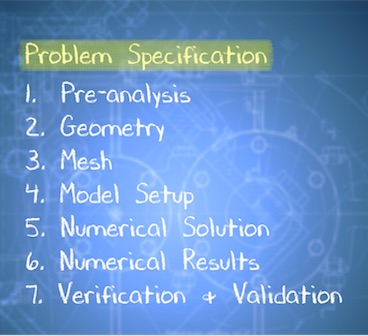
Problem Specification
This module is drawn from MAE 4230/5230 Intermediate Fluid Dynamics at Cornell University.
| Panel |
|---|
Author: Rajesh Bhaskaran, Cornell University Problem Specification |
Problem Specification
...
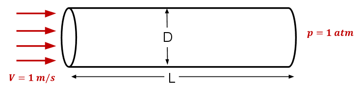
Consider fluid flowing through a circular pipe of constant
...
radius as illustrated below. The figure is not to scale. The pipe
...
diameter D = 0.2 m and
...
length L
...
= 3 m Consider the inlet velocity to be constant over the
...
cross-section and equal to 1 m/s. The
...
pressure at the pipe outlet is 1 atm. Take
...
density ρ = 1 kg/ m
...
3 and coefficient of
...
viscosity µ = 2 x
...
10 -
...
3 kg/(
...
m*s).
...
These parameters have been chosen to get a desired Reynolds number of 100 and don't correspond to any real fluid.
We'll solve this problem numerically using ANSYS Fluent. We'll look at the following results:
Velocity vectors
Velocity magnitude contours
Pressure contours
Velocity profile at the outlet
We'll verify the results by following a systematic process which includes comparing the results with the analytical solution in the full-developed region.
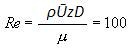
where V~avg~ is the average velocity at the inlet, which is 1m/s in this case.
Solve this problem using FLUENT. Plot the centerline velocity, wall skin-friction coefficient, and velocity profile at the outlet. Validate your results.
Note: The values used for the inlet velocity and flow properties are chosen for convenience rather than to reflect reality. The key parameter value to focus on is the Reynolds no.
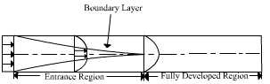
Preliminary Analysis
We expect the viscous boundary layer to grow along the pipe starting at the inlet. It will eventually grow to fill the pipe completely (provided that the pipe is long enough). When this happens, the flow becomes fully-developed and there is no variation of the velocity profile in the axial direction, x (see figure below). One can obtain a closed-form solution to the governing equations in the fully-developed region. You should have seen this in the Introduction to Fluid Mechanics course. We will compare the numerical results in the fully-developed region with the corresponding analytical results. So it's a good idea for you to go back to your textbook in the Intro course and review the fully-developed flow analysis. What are the values of centerline velocity and friction factor you expect in the fully-developed region based on the analytical solution? What is the solution for the velocity profile?
We'll create the geometry and mesh in GAMBIT which is the preprocessor for FLUENT, and then read the mesh into FLUENT and solve for the flow solution.
Go to Step 1: Create Geometry in GAMBIT